




In situ visualization reveals the magnetization reversal behavior of shape-anisotropic nanostructures
 0
0 Abstract
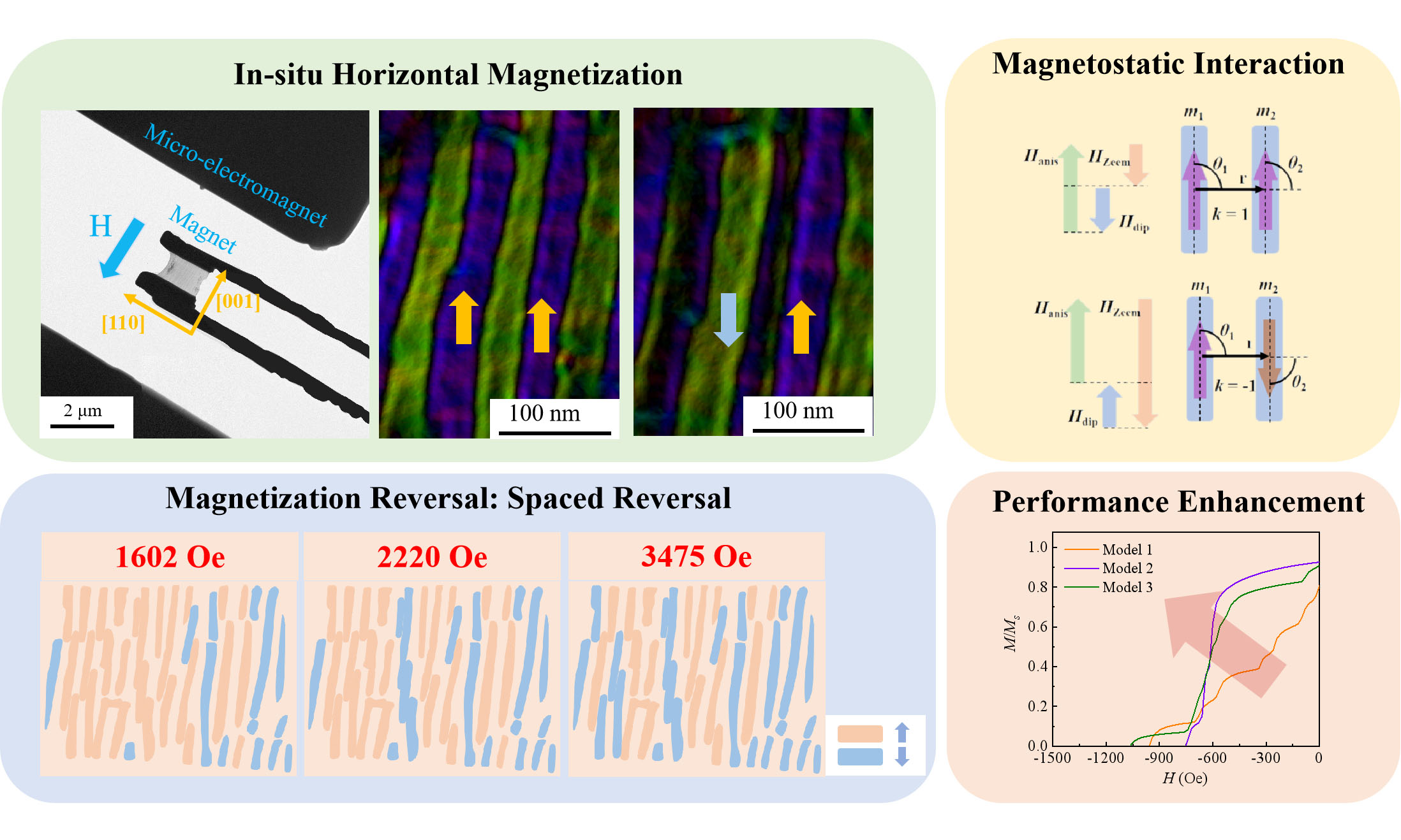
Magnetic materials dominated by shape anisotropy constitute an indispensable category of functional materials in scientific research and industrial applications. Beyond the switching field of the phases (nanowires) themselves, long-range magnetostatic interactions exert a fundamental influence on their magnetization mechanisms and modulate their overall performance. This study comprehensively investigates the role of magnetostatic interactions in the magnetization reversal process of nanowire arrays. To achieve this, the in situ horizontal magnetic field was observed using Lorentz transmission electron microscopy to investigate the magnetization reversal behavior of nanowire arrays. For the first time, the clear and precise microstructures of nanowires and the corresponding magnetization curves of target microscopic regions were acquired. In addition, the significance of magnetostatic interactions was clarified via combination with theoretical analyses. First-order reversal curve analysis, Henkel curve analysis of the macroscopic bulk material, and micromagnetic simulations were conducted to further investigate these interactions. The experimental and theoretical results show that modulating the strength of these interactions via the structural regulation of the phases (nanowires) facilitates the achievement of magnetic materials with tailored properties.
Keywords
INTRODUCTION
Shape anisotropy serves as the source of coercivity in material systems including magnetic nanowires[1-5], Alnico permanent magnets[6-9], and certain high-entropy magnets[10]. These typical shape-anisotropic magnetic materials are composed of oriented, elongated ferromagnetic units, and have been widely applied in high-density magnetic storage, high-precision sensors, and diverse permanent magnetic devices[11]. The inherent magnetization switching behavior of individual structural units is primarily governed by shape-induced demagnetization energy barriers, which pin magnetic moments along specific orientations. Nevertheless, long-range magnetostatic interactions between adjacent nanostructures act as a critical extrinsic factor[2,3]. Such inter-nanostructure coupling can profoundly alter collective magnetization reversal dynamics and ultimately determine core macroscopic magnetic parameters including coercivity, remanence squareness, and the maximum energy product. Clarifying the inherent correlation between nanoscale magnetostatic coupling and dynamic magnetization evolution is not only essential to uncover the fundamental magnetic mechanisms of anisotropic magnetic systems, but also provides a solid foundation for the targeted microstructural design and performance optimization of these widely used functional materials.
At present, the exploration of magnetostatic interactions and magnetization behaviors in anisotropic magnetic systems mainly relies on two technical routes: macroscopic magnetic characterization and micromagnetic simulation. While conventional bulk testing methods such as first-order reversal curve (FORC) analysis and Henkel plots can effectively evaluate the overall interaction characteristics and statistical magnetic responses of materials[12-17], they are unable to capture the real-time magnetization state of a single nanostructure or resolve localized differences in magnetic dynamics. Consequently, micromagnetic simulation has become a powerful auxiliary tool to predict nanoscale magnetization reversal processes[18-22]. Recent studies, including that by Sarker[20], have explored the relevant magnetic mechanisms using micromagnetic simulations. These efforts have increased academic interest in this field and highlighted the necessity of direct in situ experimental observation. However, such simulation results are highly dependent on preset structural parameters, material constants, and ideal boundary conditions. Without direct in situ experimental verification, these theoretical predictions cannot fully reflect the actual microscopic magnetization behaviors. The lack of intuitive, nanoscale experimental evidence is a major bottleneck restricting the in-depth understanding of relevant microscopic mechanisms.
Realizing the direct in situ observation of magnetization reversal at the nanoscale encounters two prominent technical challenges. On the equipment side, most traditional in situ magnetization devices in conjunction with transmission electron microscopy (TEM) generate vertical magnetic fields, which cannot match the in-plane easy axis of most shape-anisotropic magnets[8]. Meanwhile, adjusting the objective lens current to change the applied field will cause electron beam distortion and resolution degradation, complicating the construction of reliable horizontal-field in situ observation systems. On the specimen-preparation side, ordered nanowire arrays require ultra-thin TEM samples with a strictly controlled thickness. Excessive sample thickness will lead to the superposition of multiple magnetic phases and obscure the signals of individual units. Additionally, in Fresnel-mode Lorentz TEM (LTEM) images, the contrast of phase boundaries is highly similar to that of magnetic domain walls, which further increases the difficulty of distinguishing individual nanostructures and tracking their magnetization evolution.
In this study, a unique horizontal magnetic field application method was designed to enable the direct observation of the magnetization reversal process in shape-anisotropic magnetic materials via LTEM. Using this approach, the magnetization reversal sequence of the phases (nanowires) was characterized, and the hysteresis loops corresponding to the microscopic observation regions were acquired. By comparing theoretical calculations with experimental results and combining this with macroscopic performance characterization, the role of magnetostatic interactions during magnetization reversal was evaluated. Micromagnetic simulations were also employed to reveal the underlying mechanism in the investigated system.
MATERIALS AND METHODS
The Alnico alloy investigated in this work possessed a nominal composition of Fe (~ 35 wt%), Co (~ 36 wt%), Ni (~ 13 wt%), Al (~ 7 wt%), Cu (~ 3 wt%), and Ti (~ 6 wt%). Bulk alloy ingots were manufactured via directional solidification. The as-cast samples were cut into small pieces and mechanically polished to remove surface defects. A standard multistep heat treatment was then conducted in which the samples were first solution-treated at 1,250 °C for 20 min and then air-cooled to room temperature (23 °C ± 2 °C). Afterward, magnetic field annealing was performed at 800 °C for 13 min under an external field of 3000 Oe. Finally, the samples underwent three-stage tempering at 650 °C for 3 h, 600 °C for 10 h, and 550 °C for 20 h to obtain the target microstructure and magnetic properties.
Ultra-thin specimens for electron microscopy were fabricated via focused ion beam (FIB) milling using a Carl Zeiss Auriga dual-beam system (Carl Zeiss, Germany). A platinum protective film was deposited on the sample surface, followed by sequential coarse and fine ion milling to obtain lamellas with a final thickness of 28 nm, with the crystal orientation calibrated to align the sample plane with the (110) crystal plane. Scanning electron microscopy (SEM) characterization, performed on the same dual-beam system, was conducted to observe the micromorphology and verify the sample thickness. TEM measurements were carried out on a JEOL F200 field-emission transmission electron microscope (JEOL Ltd., Japan) at 200 kV, to collect high-angle annular dark field (HAADF) images, selected area electron diffraction (SAED) patterns, and energy-dispersive X-ray spectroscopy (EDS) elemental distributions. In situ magnetization tests were performed using a JEM-2100F Lorentz transmission electron microscope (JEOL Ltd., Japan) fitted with a self-developed horizontal magnetic field holder. Fresnel imaging, electron holography, and transport-of-intensity equation (TIE) reconstruction were applied to analyze the magnetic domain behaviors. Vibrating sample magnetometer (VSM) measurements were conducted on a LakeShore 7410 system (LakeShore, USA) at room temperature, to obtain hysteresis loops, isothermal remanent magnetization (IRM), direct current demagnetization remanence (DCD), Henkel curves, and first-order reversal curves (FORC). Micromagnetic simulations based on the Landau-Lifshitz-Gilbert (LLG) equation were conducted using the open-source OOMMF software to further explore the effect of magnetostatic interactions on magnetization reversal.
RESULTS
Figure 1A presents a schematic of the in situ horizontal magnetization observation system. To apply a horizontal magnetic field, a microelectromagnet was fabricated via FIB processing and fixed to the front end of the LTEM sample holder. This microelectromagnet had a gap width of 6 μm and a thickness of 15 μm, enabling the application of a ~ 1 T magnetic field while ensuring that the electron beam was not excessively deflected. The sample was welded to the tip of a tungsten needle and moved in three dimensions via piezoelectric ceramics to accurately position it into the gap of the microelectromagnet.
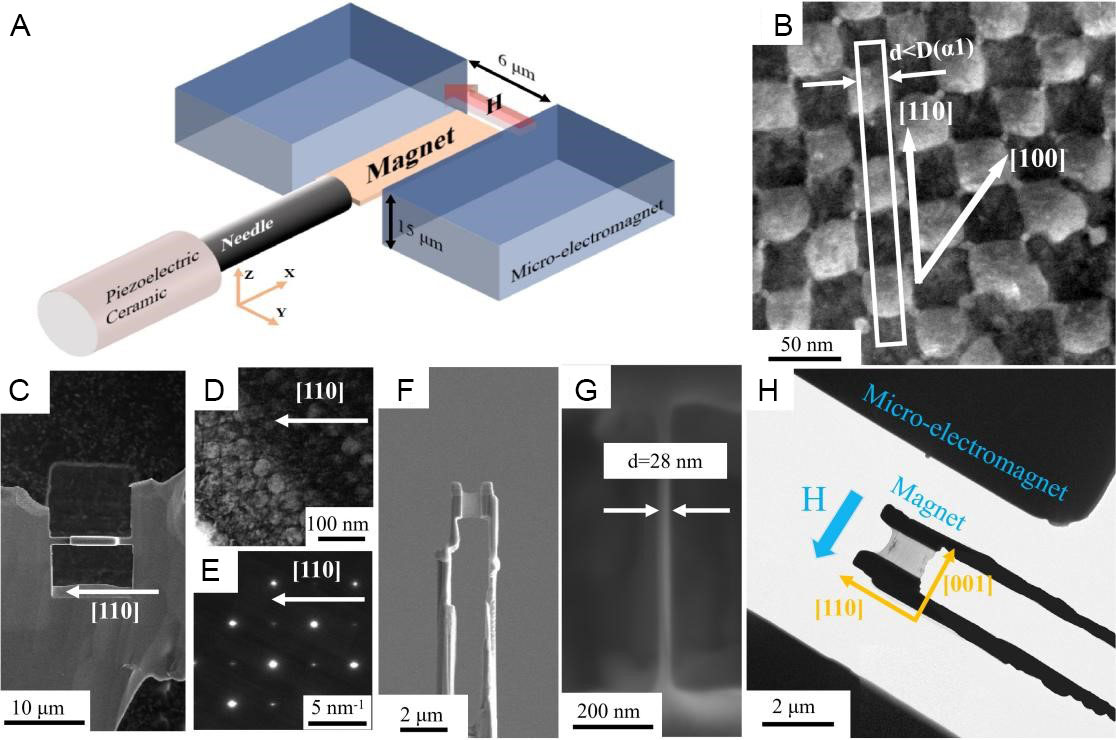
Figure 1. (A) Schematic of the in situ magnetic sample holder and SEM image of the microelectromagnet; (B) HAADF image of the Alnico alloy observed along the [001] direction, with the white box indicating the FIB sampling location; (C) SEM image of the FIB sampling area; (D) bright-field image of the FIB sampling area; (E) SAED pattern of the FIB sampling area; (F) SEM images of the samples used for in situ testing; (G) thickness of the observation area measured by SEM; (H) photograph of samples and microelectromagnets used in the In situ magnetization tests. SEM: Scanning electron microscopy; HAADF: high-angle annular dark field; FIB: focused ion beam; SAED: selected area electron diffraction.
The Alnico alloy consists of two phases formed via spinodal decomposition[23-27]. The α1 phase is a magnetic phase with a length of several hundred nanometers and a diameter of 30-40 nm. This imposes strict requirements on the thickness and orientation of the TEM samples. As shown in Figure 1B, the HAADF image acquired along the [001] zone axis demonstrates that the α1 phase forms a checkerboard-like structure with an alternating arrangement. The α1 and α2 phases are alternately arranged along the [110] direction, while the α1 phases are closely packed along the [100] direction. Therefore, the TEM samples should be oriented along the [110] direction, and their thickness should be smaller than the diameter of the α1 phases to achieve a single-layered structure. These challenges can be effectively addressed via FIB sampling performed on ion-thinned samples. The zone axis of the grain can be determined using SAED in the thin region of the ion-thinned transmission sample, as illustrated in Figure 1C and D. Without rotating the sample, we identified a region with a [001] zone axis and performed vertical sampling within the grain, as shown in Figure 1B. The sample plane obtained in this manner was parallel to the (110) crystal plane. Figure 1E presents the SAED pattern of the FIB-sampled region, while Figure 1F shows the sample used for the final in situ magnetization test. The thickness of the thin region, measured via SEM, was 28 nm (as shown in Figure 1G), which was smaller than the diameter of the α1 phases and ensured that the thin region was as close to a single-layered structure as possible while minimizing the phase overlap. Figure 1H presents an image captured during the in situ magnetization test, with the magnetic field direction parallel to the [001] direction.
Figure 2A shows a Fresnel image of the sample in the saturated remanence state, which exhibits a parallel arrangement of numerous domain walls. In the Fresnel mode, the contrasts between the α1 and α2 phases are relatively similar, such that only the α1/α2 phase interfaces can be distinguished. The morphologies of the two phases can be clearly resolved via HAADF imaging owing to the difference in atomic number between the α1 and α2 phases. Figure 2B shows the HAADF image of the sample, based on which the schematic in Figure 2C was constructed to clearly illustrate the distribution of the α1 phases. As shown in Figure 2C, most α1 phases in the rightmost region of the sample are completely isolated by α2 phases; these α1 phases exhibit considerable lengths and maintain the aspect ratios of the bulk material. In the leftmost region of the sample, a slight deviation in sample orientation leads to partial α1 phases being closely spaced, with minor overlap occurring along the thickness direction.
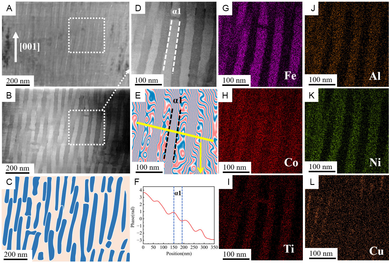
Figure 2. (A) Fresnel image of Alnico sample; (B) HAADF image of the sample; (C) two-dimensional schematic of the sample microstructure; (D) locally magnified image of the HAADF image; (E) electron holographic reconstruction image; (F) phase profile curve corresponding to the yellow line in (e); and elemental distribution maps of the local area: (G) Fe; (H) Co; (I) Ti; (J) Al; (K) Ni; (L) Cu. HAADF: High-angle annular dark field.
Figure 2D shows a locally magnified view of the HAADF image, and Figure 2E presents the electron holographic phase map of the corresponding region, while the phase profile extracted along the yellow line marked in Figure 2E is plotted in Figure 2F. The electron holographic phase map reveals that the magnetic field lines are dense within the α1 phases, indicating a relatively high saturation magnetization. By contrast, the magnetic field lines are sparse within the α2 phases, indicating significantly lower magnetization. The α2 phases function primarily to isolate the α1 phases, and the marked difference in magnetization between the two phases is a necessary prerequisite for the formation of shape anisotropy[28,29]. Further details of the electron holography acquisition are provided in Supplementary Figure 1 of the Supplementary Materials.
The saturation magnetization of the α1 phases can be precisely determined via electron holography, a key prerequisite for subsequent quantitative analysis of the magnetization reversal mechanism. When an electron beam passes through the sample, it interacts with the magnetic induction intensity (B), causing a shift in the electron phase. Magnetic induction intensity can be derived from the rate of this electron phase shift, which is defined as follows[30,31]:
where h is Planck’s constant, e is the charge of an electron, is the phase change of an electron passing through the magnetic field region, and S is the area of the magnetic flux region, which is the product of the width L of the observation region and the thickness D of the transmission sample. Based on the electron holographic measurement results, Δφ/L = 0.06 rad/nm and the sample thickness was 28 nm. The calculated saturation magnetic induction (Bs) was 14.17 kGs. Figure 2G-L present the elemental distribution maps of the corresponding region, wherein Fe and Co are shown to be enriched with the α1 phases, whereas Al, Ni, and Ti are enriched with the α2 phases. In addition, Cu is concentrated at the α1/α2 phase interfaces. This difference in elemental composition between the two phases gives rise to their distinct magnetic properties. Table 1 shows the elemental compositions of the α1 and α2 phases obtained from EDS analysis.
Elemental phase compositions (wt.%)
| Phases | Fe | Co | Al | Ni | Cu | Ti |
| α1 | 51.79 ± 8.36 | 43.41 ± 7.04 | 1.33 ± 0.39 | 2.41 ± 0.63 | 0.31 ± 0.53 | 0.75 ± 0.37 |
| α2 | 14.96 ± 2.32 | 39.53 ± 6.01 | 10.30 ± 0.92 | 21.02 ± 3.25 | 2.03 ± 0.71 | 12.16 ± 1.91 |
In situ observation of magnetic domain motion was performed on the sample depicted in Figure 2. The evolution of magnetic domains in the sample at remanence was monitored via the application of a gradually increasing reverse-applied magnetic field. Owing to the similarity between the interface contrasts of α1/α2 phases and those of domain walls in Fresnel images, determining domain directions in static images is challenging, and image processing is required to achieve more intuitive visualizations. Fresnel images at multiple focuses were also collected for verification (see Supplementary Figure 2), and dynamic contrast evolution under the applied magnetic fields confirmed that the observed features are domain walls rather than artifacts. The images in Figure 3 show a local region to illustrate the principles and procedures of image processing. The dynamic domain reversal process is provided in the Supplementary Video 1.
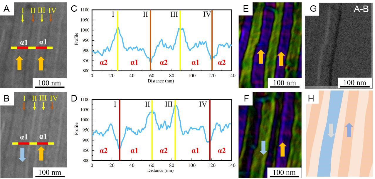
Figure 3. Local Fresnel images, contrast curves, magnetic moment distribution maps, contrast subtraction image, and schematic before and after magnetization reversal: (A) Fresnel image before magnetization reversal; (B) Fresnel image after magnetization reversal; (C) contrast variation curve corresponding to the line in (A); (D) contrast variation curve corresponding to the line in (B); (E) magnetic moment distribution map before magnetization reversal; (F) magnetic moment distribution map after magnetization reversal; (G) contrast subtraction image of (A) and (B); (H) schematic of the magnetization reversal system.
Figure 3A and B present under-focused Fresnel images captured at two distinct stages of magnetization reversal. These images show two intact α1 phases, with four domain walls (labeled I-IV) visible. Figure 3C presents the intensity profile curve corresponding to the dashed line in Figure 3A, wherein domain walls I and III appear white (corresponding to electron beam convergence regions), whereas domain walls II and IV appear black (corresponding to electron beam divergence regions). This indicates that the magnetization directions of the two α1 phases are identical. In Figure 3B, domain wall I shifts to black and domain wall II shifts to white, signaling magnetization reversal in the leftmost α1 phase. Figure 3E and F show magnetic domain images reconstructed using the TIE. Here, the magnetization direction of the leftmost α1 phase switches from upward to downward, consistent with the aforementioned analysis. This analytical approach was applied to each α1 phase throughout the magnetization process to determine their respective magnetization states. The image shown in Figure 3G was generated by subtracting the image in Figure 3A from that in Figure 3B. This difference image clearly highlights the magnetization reversal region, with other regions appearing uniform. Figure 3H provides a schematic illustrating the magnetization directions of the α1 phases based on the analysis results.
The aforementioned analysis reveals that the difference images (subtraction-based) corresponding to different applied magnetic fields during magnetization reversal clearly delineate the regions where magnetic domain reversal (MDR) occurs. Next, magnetization state diagrams under the respective magnetic fields were constructed [Figure 4]. Each α1 phase undergoes a single-domain reversal process. The reversal of internal magnetic moments within the α1 phases occurs via the curling mode. The magnetostatic interaction between the α1 phases modulates the reversal sequence, and the strength of the interaction field is dependent on the magnetization of the α1 phases and their interphase spacing. In particular, a smaller interphase spacing between α1 phases results in stronger magnetostatic interactions. Most α1 phases undergoing MDR were nonadjacent and a small number of nonreversed α1 phases were consistently present between them, resulting in an overall right-to-left alternating reversal pattern. This alternating pattern is evident in the schematics shown in Figure 4D and E, where the orange (representing downward magnetization) and blue (representing upward magnetization) regions alternate; this phenomenon is attributed to the magnetostatic interaction between α1 phases. Theoretically, for shape-anisotropic magnets, a larger aspect ratio is expected to correspond to a higher reversal field. However, this theoretical expectation was not observed in the present experiment as the overall magnetization reversal process of the sample did not follow the trend of shorter α1 phases reversing first, followed by longer ones. At an applied magnetic field of 787 Oe, two longer α1 phases underwent reversal; when the applied field reached 4,623 Oe, the leftmost α1 phase (with a small aspect ratio) had not undergone reversal. For nanowire-based structures, the presence of interphase magnetostatic interactions leads to significant differences in the switching field of nanowires between isolated and aggregated states. Detailed measurement procedures for the magnetic field strength of the micro-electromagnet are presented in Supplementary Figures 3-5 of the Supplementary Materials.
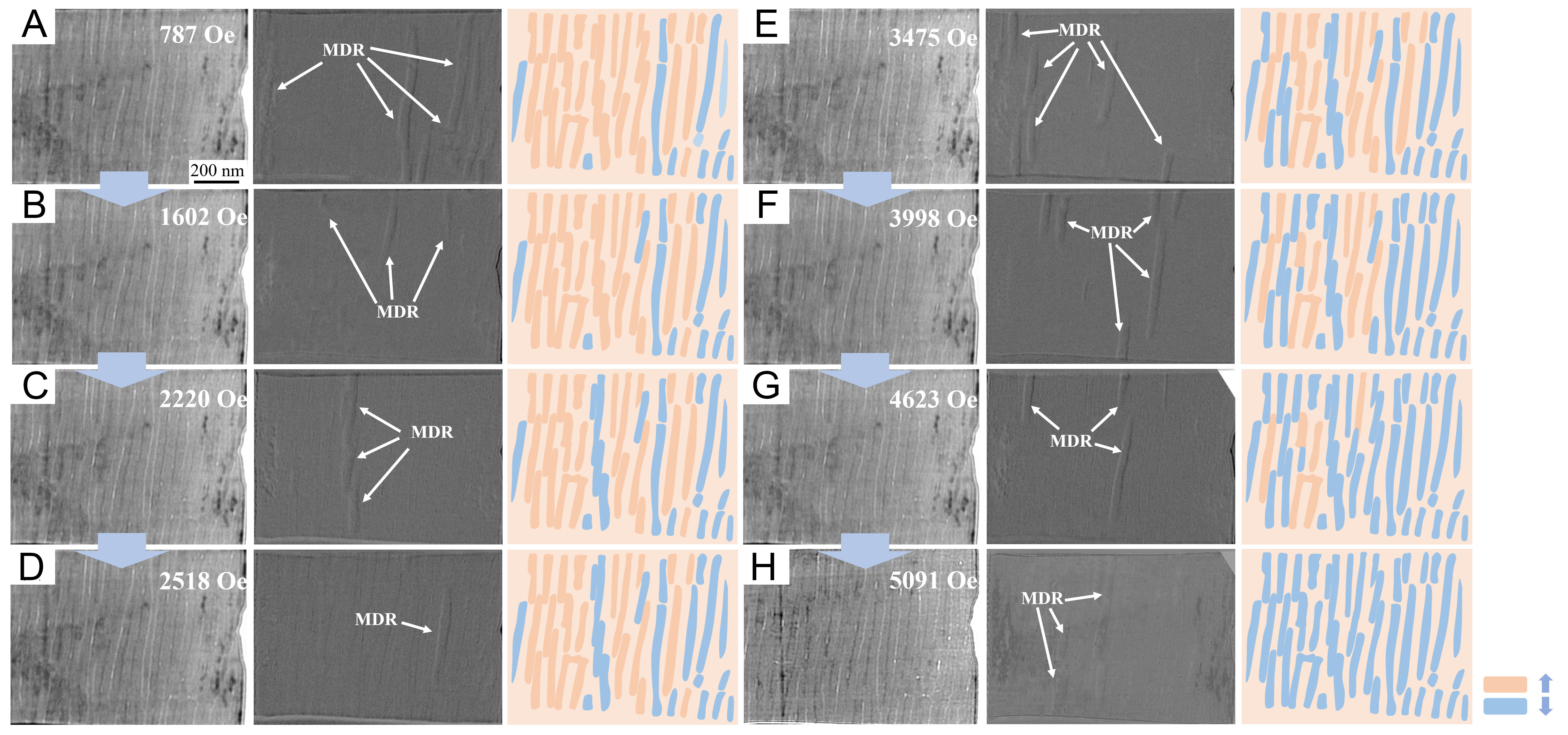
Figure 4. In situ magnetic domain evolution of the sample under increasing applied magnetic fields. (A-H) correspond to applied fields of 787 Oe, 1,602 Oe, 2,220 Oe, 2,518 Oe, 3,475 Oe, 3,998 Oe, 4,623 Oe, and 5,091 Oe, respectively. For each panel, the left column shows the original Fresnel image, the middle column marks the positions of magnetic domain reversal (MDR), and the right column presents the corresponding schematic diagram. Orange and blue regions represent magnetic domains with magnetization directions antiparallel and parallel to the applied field, respectively. All micrographs share the same scale bar.
The volume fraction of magnetization reversal under different applied magnetic fields was statistically analyzed, and the hysteresis loop corresponding to the experimentally observed region was acquired. Figure 5 presents a comparison between the hysteresis loop of the bulk alloy and that of the experimental sample. The bulk alloy exhibited a coercivity of 1,795 Oe with a symmetric hysteresis loop. By contrast, the hysteresis loop of the micro-sample shows obvious asymmetry along the field axis, with absolute coercive fields of 3,484 Oe for the descending demagnetization branch and 2,668 Oe for the ascending magnetization branch. Two primary factors contribute to this discrepancy. First, the experimental sample was extracted from a single grain, where the easy axes of all α1 phases are aligned. By contrast, bulk alloys contain multiple grains, wherein the inconsistency in grain orientation and presence of grain boundaries result in structural inhomogeneities, which in turn reduce coercivity and remanence. Second, as illustrated in Figure 1B, the spacing of α1 phases varied between the [110] and [001] directions. Specifically, the interphase spacing in the experimental sample was significantly larger than that in the bulk alloy, thereby weakening the magnetostatic interaction between α1 phases. These two factors collectively lead to the observed differences in hysteresis loops between the two samples. In situ magnetization tests were conducted to accurately characterize the relationship between the morphology of the α1 phase and the magnetization reversal sequence in the Alnico alloy, and the correlation between the microstructure and magnetization was established. It was found that the demagnetization behavior of Alnico alloy is jointly governed by the switching fields of the α1 phases and the interactions among them. The role of magnetostatic interactions between α1 phases in the demagnetization process will be considered in the following section.
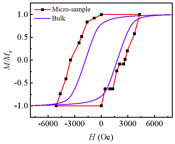
Figure 5. Hysteresis loops of Alnico magnets and those calculated from the in situ magnetization tests. The purple curve represents the bulk alloy; the red curve with square markers corresponds to the micro-sample. Both magnetization values are normalized to the saturation magnetization (M/Ms).
DISCUSSION
Henkel plots are used to identify the type of interaction present in magnets. They can be obtained by testing the IRM curve and the DCD curve according to the following formula:
If the value of ΔM is negative, the magnetostatic interaction is dominant in the material; if ΔM is positive, the exchange coupling is dominant. Figure 6A shows the IRM and DCD curves of the investigated system, while Figure 6B shows the Henkel plots. It can be seen that the magnetostatic interaction plays a major role in the applied magnetic field range of 0-5,000 Oe in the sample. As the magnetic field increases, the interaction field shows a trend of first increasing and then decreasing. When the applied magnetic field was 1,750 Oe, the interaction was the strongest.
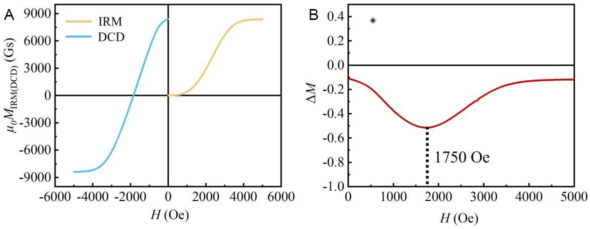
Figure 6. (A) IRM curve and DCD curve of the Alnico alloy; (B) ΔM curve of the Alnico alloy. IRM: Isothermal remanent magnetization; DCD: direct current demagnetization remanence.
The FORCs of the Alnico alloy were measured [Figure 7]. Figure 7A presents the measured FORC family, while Figure 7B shows the corresponding FORC diagram, which shows the distributions of coercive fields (Hc) and interaction fields (Hu) within the magnet[32-35]. The measurement was conducted with a magnetic field step of 100 Oe, across the full field range from positive saturation to negative saturation. The raw FORC data were processed using the VARIFORC algorithm implemented in FORCinel software, with a smoothing factor (SF) of 3 to balance noise reduction and preservation of intrinsic distribution features. For analysis, the sample was treated as an assembly of magnetic entities (i.e., α1 phases), each undergoing a single-domain reversal process and possessing unique switching and interaction fields. The three stars in the FORC diagram [Figure 7B] are used as examples to illustrate the magnetization behavior associated with the different regions of the diagram, and the corresponding schematic hysteresis loops are shown on the right-hand side. The yellow star corresponds to Hu = 0, indicating that the associated magnetic entities have no net interaction field. Here, the forward and reverse switching fields (H1 and H2) are symmetric about zero, and their magnitude is equal to the coercive field (Hc). By contrast, the hysteresis loops of the entities corresponding to the red and blue stars are shifted to the right or left, respectively, due to the influence of positive or negative Hu values, respectively. The color intensity in the FORC diagram correlates with the number of magnetic entities exhibiting a specific combination of Hc and Hu, wherein darker regions indicate a higher density of such entities. The FORC diagram of the Alnico magnet exhibits a well-defined, single-peak profile, with relatively concentrated distributions of both coercive and interaction fields. When the applied magnetic field approaches the coercivity of the investigated sample, the FORC distribution along the Hu axis becomes elongated, signifying an increase in the magnitude of the interaction fields. Near the coercivity of a magnet, the number of forward and reverse magnetic domains is balanced, at which point magnetostatic interactions between adjacent domains become the most pronounced[36,37]. The FORC diagram was used to derive the coercivity and interaction field distributions, which are shown in Figure 7C and D, respectively. The coercivity distribution confirms the presence of the dominant peak at 1,824 Oe with a distribution width of 683 Oe. Meanwhile, the interaction field distribution shows a peak centered near zero at 51 Oe with a broader distribution width of 1,990 Oe, reflecting moderate magnetostatic interactions between the magnetic phases.
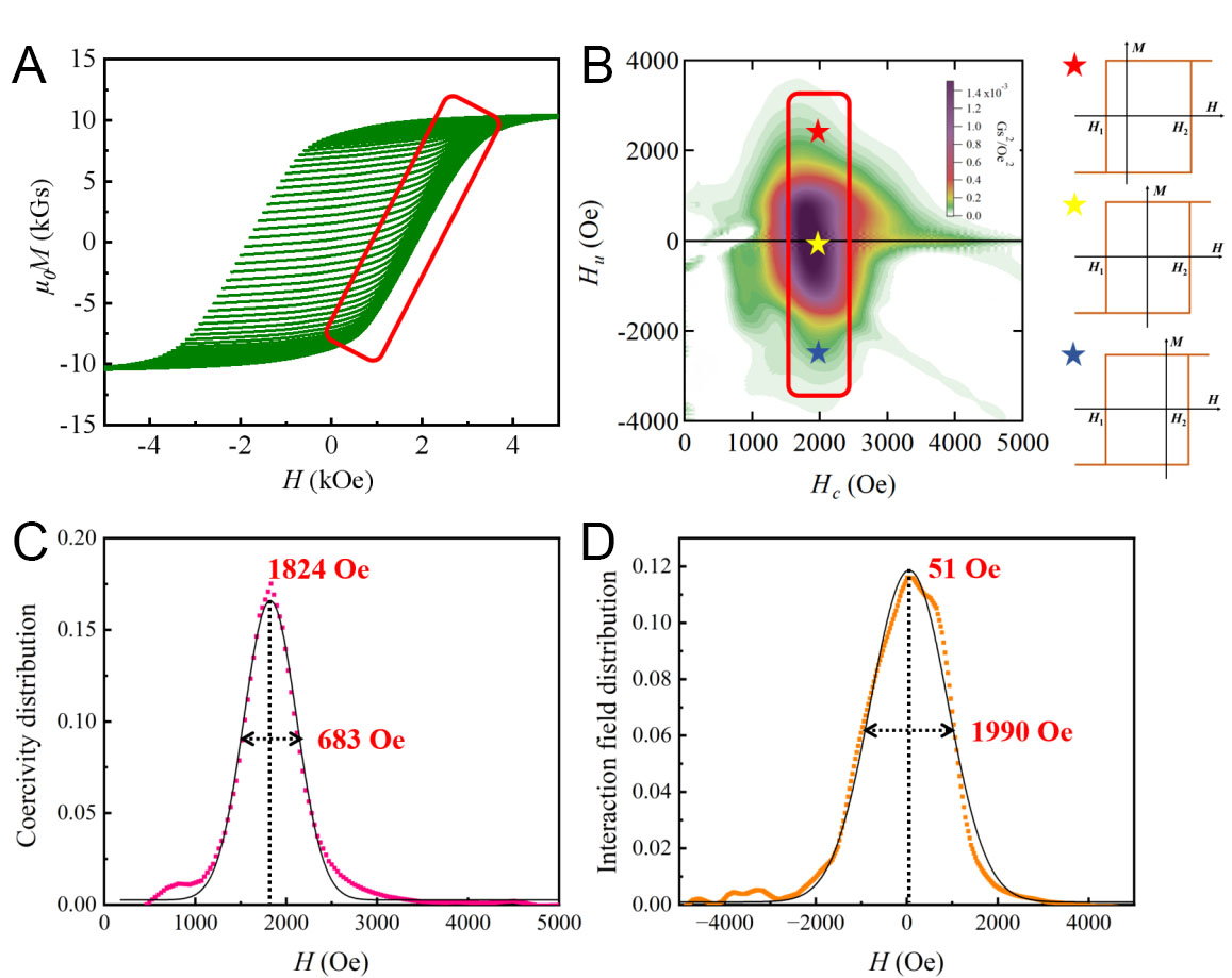
Figure 7. First-order reversal curve (FORC) analysis of the Alnico 8 magnet. (A) Measured FORC family, with the region of interest highlighted by the red rectangle; (B) FORC contour plot, where the color scale represents the FORC distribution intensity; (C) Coercivity distribution derived from the FORC diagram (D) Interaction field distribution derived from the FORC diagram.
Two factors affect the magnetization reversal process of the magnet: the reversal field of the nanowire itself and the interaction between the nanowires. According to the research[9], the magnetization reversal mechanism of α1 phase is related to the radius (R) of α1 phase When R is less than the critical radius (Rcoh), coherent rotation is present; when R is greater than Rcoh, the system is a curling model. The Rcoh of the α1 phase was 6-10 nm, and their radii (15–20 nm) are larger than this critical radius. Therefore, the curling model is more consistent with the α1 phase investigated in this study[30]. The switching field of a single α1 phase conforms to[9]:
where K is the magnetocrystalline anisotropy constant, which is often considered negligible in Alnico; N is the longitudinal demagnetization factor; R is the radius of the α1 phase; c is constant related to specimen geometry, 6.678 for a needle and A is the exchange constant. The influencing factors of the switching field are the saturation Ms, aspect ratio (demagnetization factor N), and α1 phase radius R. As the Ms value of the α1 phase in this study was constant, the demagnetization factor and radius determined the difference in the coercive field. The length and radius of each α1 phase in the sample were determined, and their demagnetization factors were calculated. In addition, switching field of each α1 phase was calculated using Equation (3). The magnetization reversal curve was then obtained according to the volume fraction, and it is shown in Figure 8. It should be noted that the longitudinal demagnetization factor N in Equation (3) was derived from the classic model of an isolated ellipsoidal particle and does not consider the mean-field effects of the dense α1 phase array. In practice, the α1 phases in a thin TEM specimen are closely packed and interact with each other, which deviates from the ideal isolated state. In this study, this approximation was adopted to distinguish the contributions of intrinsic shape anisotropy and long-range magnetostatic interactions. Accordingly, the obvious difference between the theoretical and experimental curves shown in Figure 8 quantitatively reflects the influence of the interphase magnetostatic interactions on the overall demagnetization behavior of this system. A comparison of the theoretical and experimental magnetization reversal curves shows that when the magnetic field is lower than 2,400 Oe, the theoretical M value is higher than the experimental value. By contrast, when the magnetic field is higher than 2,400 Oe, the theoretical M value is smaller than the experimental value. This difference occurs because the interaction differently affects the investigated system at different magnetizations of the magnet. In the near-saturation state, magnetostatic interactions align the magnetization of the adjacent α1 phase in an opposite direction. Therefore, the experimental value of M is lower in this system. When an adequate amount of α1 phases have been reversed, the magnetostatic interactions prevent the reversal of the unreversed α1 phase. Therefore, the experimental value of M is higher under larger applied magnetic fields.
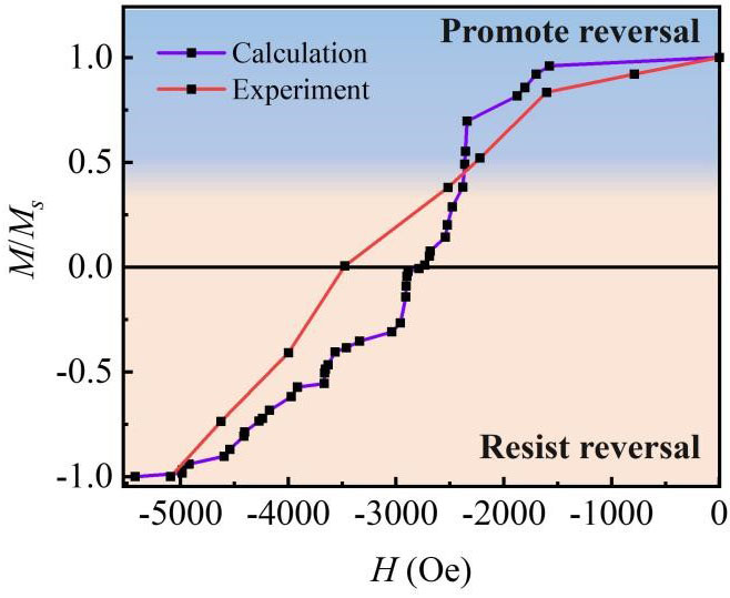
Figure 8. Experimental and theoretical demagnetization curves of the in situ magnetized samples.
The strength of the magnetostatic interaction in a shape-anisotropic magnet can be adjusted by adjusting the distance between the phases. Next, we investigated the influence of the interaction strength on the magnetization reversal process using micromagnetic simulations considering three models [Figure 9A]. The volume ratios of the α1 and α2 phases were 4:1 in Model 1, 1:1 in Model 2, and a mixed configuration of the two ratios in Model 3. The parameters used in the simulation and their sources are listed in Table 2. Figure 9B shows the demagnetization curves of the three models, and Figure 9C shows the magnetic moment diagram of the reversal process. In Model 1, when the reverse magnetic field was small, multiple α1 phases began to reverse at the same time. As the magnetic field increased, the subsequent reversal was dominated by the α1 phase magnetization reversal. By contrast, Model 2 demonstrated an independent reversal of each α1 phase from the beginning. In Model 3, the reversed α1 phase exhibited the nearest spacing among all α1 phases within this system. As the magnetic field increased, the remaining α1 phase with large spacing was reversed, and, finally, an unreversed α1 phase was present in the small-spacing region at the final magnetization. Comparing the demagnetization curves of the three models, the main difference is the squareness. The magnetization of Model 1 decreased under a small magnetic field, while those of Models 2 and 3 rapidly decreased under larger magnetic field, which results from the difference in the interaction. The minimum α1 phase spacing of Model 1 exhibited the strongest magnetostatic interaction, and the α1 phase was more prone to existing in an antiparallel state. By comparison, the interaction in Model 2 was weaker due largely to the effect of the reversal field of the α1 phase; therefore, Model 2 exhibited better squareness. This mechanism is further verified via the reversal process observed in Model 3. Here, the region exhibiting strong interactions first reverses, but after undergoing partial reversal, the interaction increases the reversal field of the unreversed component, resulting in the final complete reversal of the region.
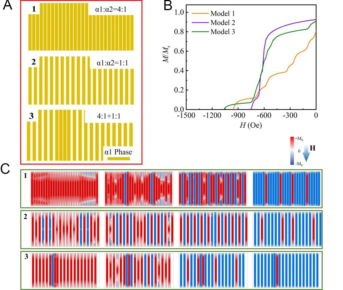
Figure 9. (A) Model of the micromagnetic simulation; (B) reverse magnetization curves of the three models from the micromagnetic simulation; (C) micromagnetic simulation results of the magnetization reversal process of the three models.
Parameters used in micro-magnetic simulation and their corresponding sources
The schematic shown in Figure 10 demonstrates the fundamental mechanism of the magnetostatic interaction as it affects the α1 magnetization reversal process. For an α1 phase (nanowire) in the array, its magnetic energy is the sum of the Zeeman, shape anisotropy, and magnetostatic interaction energies[38-41]:
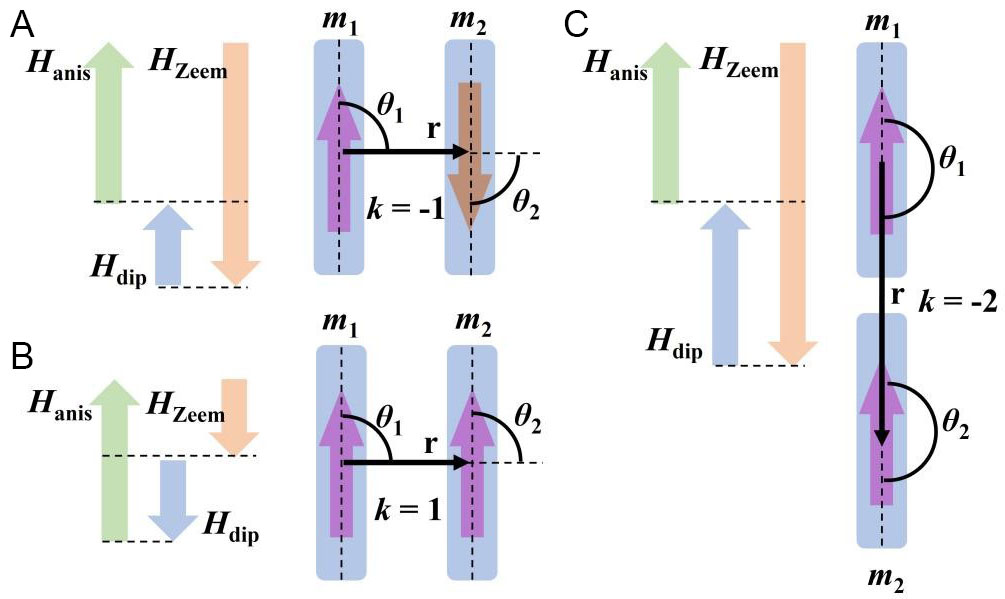
Figure 10. The schematic diagram of the principle of the influence of the magnetostatic interaction on the α1 phase switch field. (A) Schematic of two adjacent α1 phases with antiparallel magnetic moments (corresponding to k = -1); (B) Schematic of two adjacent α1 phases with parallel magnetic moments (corresponding to k = 1); (C) Schematic of two α1 phases collinearly arranged along their long axis (corresponding to k = -2).
where m is the magnetic dipole moment, and r is the direction vector between the magnetic dipoles. Here, we consider two magnetic dipoles as an example, and the influence of their interactions is discussed. Their interaction energy is defined as:
where φ is the angle between two magnetic dipoles, and θ is the angle between m and r. Let k = cosφ - 3cosθ1cosθ2. Here, two adjacent α1 phases are considered to be two magnetic dipoles. When the magnetic moment directions of the two particles are parallel, k = 1 and the direction of the interaction field Hdip is the same as that of the applied magnetic field HZeem. In this system, only a small applied magnetic field is needed to overcome the anisotropy field Hanis. When the magnetic moment directions of the two particles are antiparallel, k = -1 and the direction of Hdip is opposite to that of HZeem. In this context, HZeem needs to overcome the sum of Hanis and Hdip, and therefore the switching field is larger. This leads to the exchange bias characteristics demonstrated in the α1 phases hysteresis loop. For two particles on the same line in the long axis direction, as shown in Figure 10C, we obtain k = -2. This leads to a larger Hdip value, and the magnetostatic interaction increases the switching field of the particles.
According to the above analysis, the existence of the magnetostatic interaction in a nanowire array results in a significant change in the switching field, which affects the magnetization reversal process of the system. The magnetostatic interaction reduces the switching field at the beginning of the magnetization reversal process and increases the switching field when the magnetic field increases to a certain value, thereby reducing the squareness and maximum magnetic energy product of the system. Therefore, tuning the position and distance of the phase in the nanoarray can effectively alter the magnitude and distribution of the interaction field and regulate the performance of the magnet.
CONCLUSION
The microstructure and magnetic domain reversal process of a nanowire array structure were investigated using LTEM. Each phase (nanowire) is a single-domain reversal mode. Magnetostatic interactions cause the nanowire array structure to undergo alternating reversal. The Henkel curve and FORC analysis confirmed that magnetostatic interactions greatly affect this reversal process, and the interaction field was the strongest when partial demagnetization was observed. The hysteresis loop of the system without considering magnetostatic interactions was obtained via theoretical calculations. A comparison with the experimental results revealed that the magnetostatic interaction leads to a faster decrease in magnetization in the early stage and a slower decrease in magnetization after undergoing partial demagnetization. Micromagnetic simulations were also conducted, which demonstrated that enhanced interactions lead to a decrease in squareness and a lower maximum magnetic energy product. Our findings indicate that the distance between phases (nanowires) can be adjusted to control the strength of the interaction field and improve the performance of magnetic materials.
DECLARATIONS
Authors’ contributions
Made substantial contributions to conception and design of the study: Zhao, Z.; Zhao, J.
Performed data analysis and interpretation: Zhao, Z.; Jiang, L.; Sun, Y.
Performed data acquisition: Liu, L.; Yu, X.; Ding, Y.; Xia, W.
Provided administrative, technical, and material support: Xia, W.; Jiang, L.; Sun, Y.
Drafted and critically revised the manuscript for important intellectual content: Zhao, Z.; Zhao, J.; Yan, A.
Final approval of the version to be published: Zhao, Z.; Zhao, J.; Liu, L.; Yu, X.; Ding, Y.; Xia, W.; Jiang, L.; Sun, Y.; Yan, A.
Availability of data and materials
The data supporting the findings of this study are available within this Article and its Supplementary Materials. Further data are available from the corresponding authors upon request.
AI and AI-assisted Tools statement
Not applicable.
Financial support and sponsorship
This work was supported by the National Key R&D Program of China (No.2022YFB3807900), Youth Innovation Promotion Association CAS (2023311), and Youth Science and Technology Innovation Leading Talent Project of Ningbo (2024QL002).
Conflicts of interest
All authors declared that there are no conflicts of interest.
Ethical approval and consent to participate
Not applicable.
Consent for publication
Not applicable.
Copyright
© The Author(s) 2026.
Supplementary Materials
REFERENCES
1. Shrivastava, S. K.; Agarwal, S.; Abushuhel, M.; et al. Diameter and temperature dependent structure and magnetic properties of electrodeposited CoNiCu alloy nanowires. J. Supercond. Nov. Magn. 2026, 39, 7199.
2. Jiang, Y.; Feng, J.; Liu, G.; et al. A Novel Method for identifying the magnetic interaction and reversal mechanisms in nickel nanowires using FORC diagrams and micromagnetic slicing. J. Supercond. Nov. Magn. 2025, 38, 6958.
3. Samardak, A.; Nasirpouri, F.; Nadi, M.; et al. Conversion of magnetic anisotropy in electrodeposited Co-Ni alloy nanowires. J. Magn. Magn. Mater. 2015, 383, 94-9.
4. Sampaio, L. C.; Sinnecker, E. H. C. P.; Cernicchiaro, G. R. C.; Knobel, M.; Vázquez, M.; Velázquez, J. Magnetic microwires as macrospins in a long-range dipole-dipole interaction. Phys. Rev. B. 2000, 61, 8976-83.
5. Terruzzi, P.; Alburquenque, D.; Saavedra, E.; Escrig, J. Magnetic properties of cobalt nanofibers synthesized via electrospinning and thermal treatment: Implications for nanoscale device applications. Chin. J. Phys. 2026, 101, 515-23.
6. Rehman, S. U.; Du, Z.; Yang, M.; et al. Evolution of microstructure and magnetic properties in Alnico 6 magnets under various processing conditions. J. Alloy. Compd. 2026, 1051, 185980.
7. Zhou, M.; Sun, J.; Zhang, H.; Chi, X.; Ding, H.; Wang, Y. Preparation of Alnico alloy with high magnetic properties by the two-phase composite method. J. Alloy. Compd. 2025, 1039, 183272.
8. Zhou, L.; White, E.; Ke, L.; et al. Microstructure and coercivity in alnico 9. J. Magn. Magn. Mater. 2019, 471, 142-7.
9. Zhou, L.; Miller, M.; Lu, P.; et al. Architecture and magnetism of alnico. Acta. Materialia. 2014, 74, 224-33.
10. Chen, H.; Gou, J.; Jia, W.; Song, X.; Ma, T. Origin of hard magnetism in Fe-Co-Ni-Al-Ti-Cu high-entropy alloy: chemical shape anisotropy. Acta. Materialia. 2023, 246, 118702.
11. Subba, D.; Srinivasan, A. Assessment of X-type Fe2CoAl nanowires synthesized by electrospinning route for advanced magnetic applications. J. Alloy. Compd. 2025, 1035, 181513.
12. Sahu, S.; Koteswara, Rao. B.; Sahoo, S. K.; Narayana, Jammalamadaka. S.; Basheed, G. Influence of post-annealing on magnetic anisotropy, magnetic domain-state configuration and broadband ferromagnetic resonance in Co60Fe20B20 thin films. J. Magn. Magn. Mater. 2026, 648, 174085.
13. Han, M. FORC and Mössbauer techniques disclosed multiple losses origins in FeCuNbSiB microwire composites with remarkable microwave absorption. J. Alloy. Compd. 2026, 1061, 187533.
14. Mohammadalizadeh, M.; Tabatabaei, Fard. S. M.; Montazer, A. H.; Almasi, Kashi. M. First-order reversal curve investigation of CoFe alloy microparticles and their microwave absorption properties. J. Mater. Sci:. Mater. Electron. 2025, 36, 16331.
15. Proenca, M. P.; Sousa, C. T.; Ventura, J.; Garcia, J.; Vazquez, M.; Araujo, J. P. Identifying weakly-interacting single domain states in Ni nanowire arrays by FORC. J. Alloy. Compd. 2017, 699, 421-9.
16. Kouhpanji MR, Stadler BJH. Beyond the qualitative description of complex magnetic nanoparticle arrays using FORC measurement. Nano. Ex. 2020, 1, 010017.
17. Ciureanu, M.; Béron, F.; Ciureanu, P.; et al. First order reversal curves (FORC) diagrams of Co nanowire arrays. J. Nanosci. Nanotechnol. 2008, 8, 5725-32.
18. Laha, P.; Gayen, R. N.; Sabareesan, P. Magnetization reversal dynamics of electrodeposited Ni1-xFex nanowires. Solid. State. Commun. 2025, 402, 115954.
19. Mel’nikov, G. Y.; Burban, E. A.; Svalov, A. V.; Yushkov, A. A.; Kurlyandskaya, G. V. Core-shell α-Fe/FeOx nanoparticles synthesized by electrical explosion of a wire and ball milling. experience in the development of a micromagnetic digital twin. Phys. Metals. Metallogr. 2025, 126, 1435-43.
20. Sarker, S.; Rajib, M. M.; Barua, R.; Atulasimha, J. Theoretical limits for energy density of aligned ferromagnetic nanoparticles in a nonmagnetic matrix for rare-earth-free permanent magnets. Appl. Phys. Lett. 2025, 126, 092404.
21. Vieira, G. B.; Howard, E.; Lankapalli, P.; Phillips, I.; Hoffmeister, K.; Holley, J. Stray magnetic field variations and micromagnetic simulations: models for Ni0.8Fe0.2 disks used for microparticle trapping. Micromachines. (Basel). 2024, 15, 567.
22. Jalal, E. M.; Bokpe, D.; Kerrai, H.; et al. Monte Carlo study of compensation temperature and hysteresis behavior in a cylindrical ferrimagnetic Ising nanowire. Appl. Phys. A. 2026, 132, 9679.
23. Wu, Q.; Sun, Z.; Pan, A.; et al. Tailoring microstructure orientation and magnetic properties in AlNiCo permanent magnets by controlled withdrawal rate in high-rate solidification. Magnetochemistry 2026, 12, 43.
24. Cui, J.; Kramer, M.; Zhou, L.; et al. Current progress and future challenges in rare-earth-free permanent magnets. Acta. Materialia. 2018, 158, 118-37.
25. Bishop, O.; Duong, A.; Smith, I.; Snyder, K.; Carpenter, E.; Barua, R. Magnetic-field-assisted directed energy deposition processing of Alnico for enhanced coercivity and magnetic anisotropy. AIP. Advances. 2026, 16, 025038.
26. Ahmad, Z.; Liu, Z.; ul, Haq. A. Synthesis, magnetic and microstructural properties of Alnico magnets with additives. J. Magn. Magn. Mater. 2017, 428, 125-31.
27. Han, X.; Sun, J.; Liu, T.; Wang, H.; Zhang, Y.; Cui, C. Effects of magnetic field and annealing on the structure and magnetic properties of Alnico ribbons. J. Alloy. Compd. 2019, 785, 715-24.
28. Dussa, S.; Sarkar, S. K.; Verma, K. K.; et al. Thermal treatment induced nano-scale spinodal decomposition for enhanced hard-magnetic properties in laser additively fabricated Alnico-8H. Appl. Mater. Today. 2025, 44, 102679.
29. Dussa, S.; Sarkar, S. K.; Joshi, S. S.; Banerjee, R.; Dahotre, N. B. Leveraging miscibility gap via low-temperature annealing for enhanced hard magnetic properties in laser additively processed Alnico-8H. Scripta. Materialia. 2026, 271, 116996.
30. Zhu, S.; Zhao, J.; Xia, W.; Sun, Y.; Peng, Y.; Fu, J. Magnetic structure and coercivity mechanism of AlNiCo magnets studied by electron holography. J. Alloy. Compd. 2017, 720, 401-7.
31. Xia, W.; Hirata, K.; Yanagisawa, K.; et al. Quantitative evaluation of magnetic flux density in a magnetic recording head and pseudo soft underlayer by electron holography. J. Electron. Microsc. (Tokyo). 2010, 59, 331-7.
32. Egli, R. VARIFORC: An optimized protocol for calculating non-regular first-order reversal curve (FORC) diagrams. Global. Planet. Change. 2013, 110, 302-20.
33. Nica, M.; Stancu, A. FORC diagram study of magnetostatic interactions in 2D longitudinal arrays of magnetic wires. Physica. B. 2015, 475, 73-9.
34. Muscas, G.; Menniti, M.; Brucas, R.; Jönsson, P. Mesoscale magnetic rings: complex magnetization reversal uncovered by FORC. J. Magn. Magn. Mater. 2020, 502, 166559.
35. Wu, Q.; Li, J.; Ge, H.; Tu, Y.; Pan, M.; Zhang, P. Coercivity mechanism and FORC analysis of MnBi-based permanent alloy. J. Magn. Magn. Mater. 2020, 503, 166600.
36. Aslibeiki, B.; Eskandarzadeh, N.; Jalili, H.; et al. Magnetic hyperthermia properties of CoFe2O4 nanoparticles: effect of polymer coating and interparticle interactions. Ceram. Int. 2022, 48, 27995-8005.
37. Kouhpanji MR, Stadler B. Exploring effects of magnetic nanowire arrangements and imperfections on first-order reversal curve diagrams. IEEE. Trans. Magn. 2022, 58, 1-6.
38. Liu, Q.; Wang, J.; Yan, Z.; Xue, D. Characterization and magnetic properties of Fe1-xNix nanowire arrays. Phys. Rev. B. 2005, 72, 144412.
39. Samanifar, S.; Almasi, Kashi. M.; Ramazani, A.; Alikhani, M. Reversal modes in FeCoNi nanowire arrays: correlation between magnetostatic interactions and nanowires length. J. Magn. Magn. Mater. 2015, 378, 73-83.
40. Aslibeiki, B. Magnetic interactions and hysteresis loops study of Co/CoFe2O4 nanoparticles. Ceramics. International. 2016, 42, 6413-21.
Cite This Article
 Open Access
How to Cite
Download Citation
Export Citation File:
Type of Import
Tips on Downloading Citation
Citation Manager File Format
Type of Import
Direct Import: When the Direct Import option is selected (the default state), a dialogue box will give you the option to Save or Open the downloaded citation data. Choosing Open will either launch your citation manager or give you a choice of applications with which to use the metadata. The Save option saves the file locally for later use.
Indirect Import: When the Indirect Import option is selected, the metadata is displayed and may be copied and pasted as needed.
About This Article
Copyright

Data & Comments
Data
0










Comments
Comments must be written in English. Spam, offensive content, impersonation, and private information will not be permitted. If any comment is reported and identified as inappropriate content by OAE staff, the comment will be removed without notice. If you have any queries or need any help, please contact us at [email protected].