
Figure3
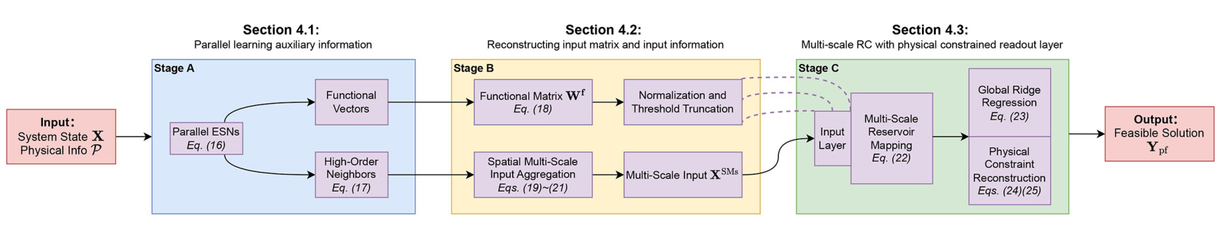
Figure 3. Flowchart summarizing the key components and equations in Sections 4.1–4.3. Section 4.1 (Stage A): Parallel learning extracts functional vectors via reservoir state evolution (Eq. 16) and identifies higher-order neighbors via Bus-Pair loss (Eq. 17). Section 4.2 (Stage B): Constructs the functional matrix (Eq. 18) and generates spatial multi-scale input via physics-informed aggregation (Eqs. 19–21). Section 4.3 (Stage C): Trains multi-scale reservoir (Eq. 22) with ridge regression (Eq. 23) and applies physical power flow constraints (Eqs. 24 and 25) to ensure feasible solutions.


