Download PDF
Research Article  |  Open Access  |  23 Apr 2026

Reinforcement learning-based attitude control for a quadrotor UAV system with performance constraints

Views: 60 |  Downloads: 5 |  Cited:  0
Intell. Robot. 2026, 6(2), 184-204.
10.20517/ir.2026.10 |  © The Author(s) 2026.
Author Information
Article Notes
Cite This Article

Abstract

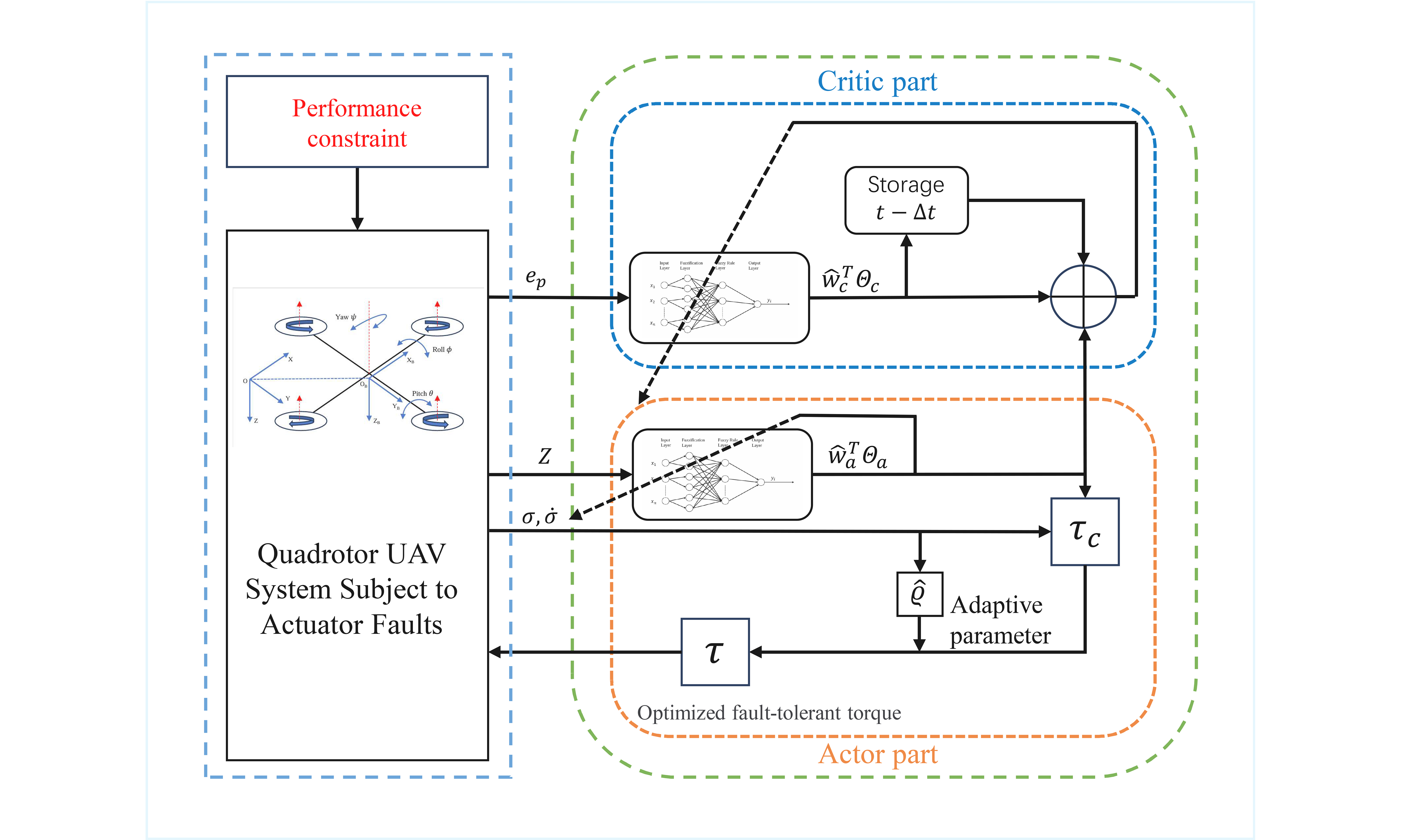
In this paper, a fuzzy logic-based fault-tolerant attitude control strategy is proposed for the attitude tracking of a quadrotor unmanned aerial vehicle (UAV) subject to actuator faults. The attitude dynamics of the quadrotor are represented using modified Rodrigues parameters. Inspired by the biological trial-and-error mechanism that reinforcement learning (RL) emulates, the proposed method is developed by integrating fuzzy logic systems (FLSs) with RL. To enhance the autonomous learning capability and tracking performance of the UAV system, actor–critic (AC) learning is introduced as an effective RL method. A cost function defined in terms of tracking errors is introduced, and an FLS is incorporated into the critic to approximate the cost function for performance evaluation. The actor is responsible for generating the control input based on the critic signals. Concurrently, another FLS is employed to approximate system uncertainties and actuator bias faults. Furthermore, to meet increasingly stringent control requirements, performance constraints are imposed to guarantee prescribed tracking performance. The system stability and convergence of tracking errors are analyzed using Lyapunov stability theory. Finally, simulations are conducted to verify the effectiveness of the proposed adaptive fault-tolerant attitude control scheme.

Keywords

Quadrotor UAV, reinforcement learning, actor-critic learning, fuzzy logic system, prescribed performance, actuator faults, adaptive fault-tolerant attitude control

1. INTRODUCTION

Inspired by the exceptional agility and adaptability of biological flyers, the development of highly autonomous and agile aerial robotics has garnered significant attention in recent years [13]. As a representative platform in this field, the quadrotor unmanned aerial vehicle (UAV) is distinguished by its compact structure, high maneuverability, and vertical takeoff and landing capability [46]. However, quadrotor UAV systems are inherently highly nonlinear, strongly coupled, and subject to significant model uncertainties [7]. In practical applications, UAV system performance can also be adversely affected by external disturbances, sensor inaccuracies, and actuator faults, which pose significant challenges for conventional control methods [8]. Intelligent adaptive control offers the advantage of strong resilience and autonomous decision-making capability, enabling the system to maintain stable performance in complex environments. Consequently, adaptive control strategies offer a promising solution to these challenges.

In practical scenarios, actuator faults have detrimental effects on quadrotor UAV operations. These faults can significantly degrade control performance and even lead to system instability or mission failure. To address the challenges, extensive research has been conducted, resulting in the development of various control strategies [911]. For instance, Zhao et al. employed reinforcement learning (RL) to obtain an optimal control policy for suppressing actuator faults [9]. Furthermore, Ma et al. proposed a distributed adaptive method that compensates for actuator faults with gain uncertainties and structural changes, which can ensure stable UAV–unmanned ground vehicle (UGV) formation [11]. However, most existing methods rely on accurate models and primarily focus on efficiency loss, while neglecting concurrent bias faults. Thus, it is essential to develop fault-tolerant control schemes capable of addressing simultaneous multiplicative and additive faults.

Fuzzy logic systems (FLSs) are suitable for uncertain and highly nonlinear systems, because they can approximate complex nonlinear functions without requiring an accurate mathematical model. Moreover, their rule-based structure provides interpretability and flexibility in controller design, which facilitates the effective handling of external disturbances and system uncertainties [1214]. Zhang et al. employed an FLS to approximate unknown nonlinear dynamics over a compact set within an ideal controller framework [15]. Additionally, Yu et al. utilized an FLS to approximate unknown nonlinearities and estimate unmeasurable states, achieving finite-time probabilistic stability under stochastic disturbances [16]. Consequently, FLS can serve as an effective tool for addressing model uncertainties and complex nonlinear dynamics in quadrotor UAV systems.

As a key realization of biomimetic intelligence, RL mimics the trial-and-error learning capability of biological systems[1719]. Through continuous interaction with the environment, RL can learn control policies online, thereby enhancing decision-making performance. To meet the increasing demand for autonomy and intelligence, actor–critic (AC) learning has emerged as an effective RL-based approach. This method employs a specialized architecture consisting of two interacting networks that evaluate the value function and optimize the control policy, enabling online adaptive control [2023]. For example, Ouyang et al. proposed an adaptive coordinated control method based on an AC framework to address the optimal tracking control problem of dual-arm robots [24]. Similarly, AC learning has been utilized to handle unknown system uncertainties, where the critic approximates the performance cost and the actor generates compensation control [25]. In addition, odd-numbered symmetric actuators and even-numbered critics have been introduced to address instability and asymmetry problems in quadrotor flight control based on AC learning [26]. These studies demonstrate that the AC architecture, inspired by RL, can learn approximately optimal control policies through online interaction without relying on an explicit system model. As such, it significantly enhances autonomous learning and optimization performance, thereby fulfilling the overarching requirements for autonomy and intelligence.

Prescribed performance, as a class of performance constraints, addresses control tasks with explicit transient and steady-state requirements. A prescribed performance function (PPF) is commonly employed to ensure that tracking error, convergence rate, and overshoot remain within predefined bounds [2731]. For example, Yu et al. developed finite-time PPFs to transform distributed tracking errors into a new set of errors based on the transient and steady-state requirements[28]. Moreover, Li et al. integrated an improved performance function with a reduced-order K-filter to realize prescribed performance while relaxing initial state constraints [31]. Therefore, to meet the growing need for superior attitude control performance in UAV systems, prescribed performance strategies have become increasingly attractive and viable.

In this paper, we focus on the adaptive attitude tracking control problem for a quadrotor UAV subject to actuator faults. To enhance autonomous learning and optimization performance under such conditions, an adaptive fault-tolerant attitude control method integrating an FLS with RL is proposed. Furthermore, to satisfy increasingly stringent control requirements, a prescribed performance constraint is incorporated into the UAV system. Based on the above, the main contributions of this paper are shown as follows:

1. Compared with existing RL-based control schemes for quadrotor UAVs [9,20,26], the proposed RL-based fuzzy adaptive attitude control not only achieves optimized tracking control performance under prescribed performance constraints, but also avoids the adverse effects caused by actuator faults. By employing an FLS, the proposed approach achieves faster convergence due to simpler parameter tuning and fewer training iterations. In the proposed AC-based RL architecture, the critic component evaluates future performance and yields an evaluative signal, while the actor component generates an optimized reinforced control input that compensates for system uncertainties and actuator faults.

2. Different from existing fault-tolerant control methods for quadrotor UAVs [9,11], the proposed approach considers the simultaneous occurrence of actuator efficiency degradation faults and bias faults. Accordingly, a unified fault model is constructed to characterize these concurrent failures, which facilitates effective compensation for their combined effects.

The remainder of this paper is organized as follows. Section 2 presents the preliminary concepts and problem formulation. Section 3 shows the development of the proposed RL-based fault-tolerant attitude control strategy, along with the corresponding stability analysis. Section 4 presents simulation studies to validate the effectiveness of the proposed approach. Finally, Section 5 concludes the paper.

Notation: Throughout this paper, $$ \mathbb{R} $$ denotes the set of real numbers, and $$ \mathbb{R}^n $$ denotes the n-dimensional Euclidean space. Let I denote the identity matrix. The functions $$ \lambda_\text{min}(\bullet) $$, $$ \lambda_\text{max}(\bullet) $$, and $$ \text{tr}(\bullet) $$ denote the minimum eigenvalue, maximum eigenvalue, and trace of a matrix, respectively. The notation $$ \text{diag}(\bullet) $$ represents a diagonal matrix, $$ \odot $$ stands for the Hadamard product, and $$ (\bullet)^\times $$ represents the skew-symmetric matrix associated with a vector $$ \bullet \in \mathbb{R}^3 $$. The notation $$ \|\bullet\| $$ denotes the Euclidean norm of a vector or the Frobenius norm of a matrix.

2. PRELIMINARIES

2.1. Kinematics and dynamics of the UAV attitude system with actuator faults

The structural diagram of a quadrotor UAV is shown in Figure 1, which includes two coordinate frames: the inertial frame OXYZ and the body-fixed frame $$ O_BX_BY_BZ_B $$. The orientation of the body-fixed frame relative to the inertial frame is represented by modified Rodrigues parameters (MRPs)[32]. Accordingly, the attitude kinematics and dynamics of the quadrotor UAV are described as

$$\dot{\sigma}=G(\sigma)\omega, $$

$$J\dot{\omega}=-\omega^\times J\omega+\tau_a, $$

Reinforcement learning-based attitude control for a quadrotor UAV system with performance constraints

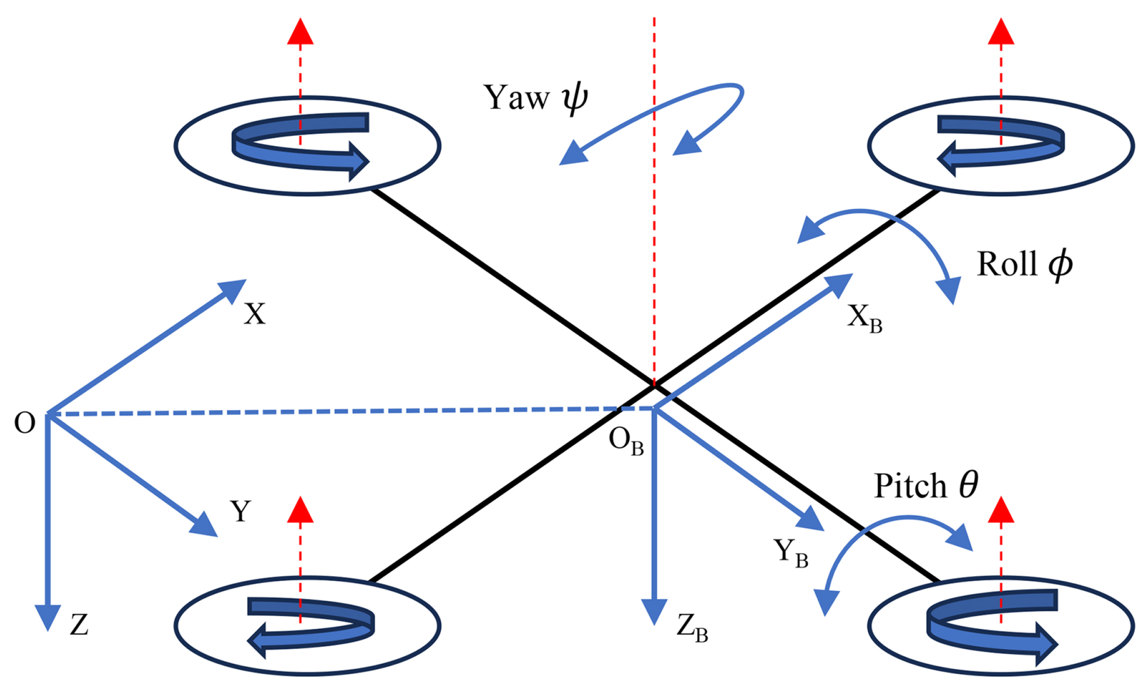
Figure 1. Structural diagram of a quadrotor UAV. UAV: Unmanned aerial vehicle.

where $$ \sigma=e $$tan$$ (\Phi/4) $$, Φ is the Euler angle, e is the Euler axis, and $$ \omega=[\omega_x, \omega_y, \omega_z]^T $$ denotes the angular velocity of the quadrotor UAV. $$ J\in\mathbb{R}^{3\times3} $$ is the inertia matrix, $$ \tau_a\in\mathbb{R}^3 $$ denotes the control torque, and the kinematic matrix $$ G(\sigma) $$ is given by

$$G(\sigma)=\frac{1}{2}\left[\frac{1-\sigma^T\sigma}{2}I+\sigma^{\times}+\sigma\sigma^T\right].$$

It should be noted that the MRP representation possesses a coordinate singularity at $$ \Phi = \pm360^\circ $$, where the term $$ \text{tan}(\Phi/4) $$ diverges. However, for the quadrotor UAV attitude control task considered in this study, the rotation angle Φ is assumed to remain within a restricted operating region $$ (|\Phi|<360^\circ) $$, which is well-suited for most flight maneuvers. Under this condition, the MRPs provide a more compact and efficient parameterization compared to quaternions or Euler angles, and the singularity issue can be effectively avoided through proper initial condition settings and performance constraints. Therefore, Equations (1) and (2) can be reformulated as

$$M(\sigma)\ddot{\sigma}+C(\sigma, \dot{\sigma})\dot{\sigma}=\tau, $$

where

$$M(\sigma)= G^{-T}(\sigma)JG^{-1}(\sigma), $$

$$C(\sigma, \dot{\sigma})= -G^{-T}JG^{-1}\dot{G}G^{-1} - G^{-T}(J\omega)^{\times}G^{-1}, $$

$$\tau= G^{-T}(\sigma)\tau_a, $$

which satisfy the following properties.

Property 1[32]. $$ M(\sigma) $$ is bounded as follows:

$$0<k_m\|\sigma\|^2 \leq \sigma^T M(\sigma) \sigma \leq k_n\|\sigma\|^2, \quad \forall \sigma \in \mathbb{R}^3$$

where $$ k_m $$ and $$ k_n $$ are positive constants.

Property 2[33]. $$ \dot{M}(\sigma)-2C(\sigma, \dot{\sigma}) $$ is skew-symmetric. For the skew-symmetric matrix $$ \dot{M}(\sigma)-2C(\sigma, \dot{\sigma}) $$, it holds that $$ \zeta^T(\dot{M}(\sigma)-2C(\sigma, \dot{\sigma}))\zeta=0 $$, with $$ \zeta\in\mathbb{R}^{3} $$.

In this paper, the actuator fault model, which encompasses efficiency loss and bias-type faults, is expressed as[34]

$$\tau_{f, i}(t)=(1-\kappa_i)\tau_i(t)+\tau_{o, i}(t), \ \ t\geq t_i$$

where $$ \tau_i(t) $$ is the designed control input, $$ \kappa_i $$ is an unknown variable in the range [0, 1) representing loss of control effectiveness. The positive loss matrix is defined as $$ \kappa_f=\text{diag}(1-\kappa_1, ..., 1-\kappa_n)\in\mathbb{R}^{n\times n} $$. $$ \tau_o(t)=[\tau_{o, 1}(t), \tau_{o, 2}(t), \tau_{o, 3}(t)]^T $$ is the unknown bias fault function. Here, $$ t_i $$ represents the failure time of each actuator.

By incorporating Equation (9) into Equation (4), the system dynamics under actuator faults can be rewritten as

$$M(\sigma)\ddot{\sigma}+C(\sigma, \dot{\sigma})\dot{\sigma}=\kappa_f\tau(t)+\tau_{o}(t), $$

where $$ \tau=[\tau_1, \tau_2, \tau_3]^T $$ denotes the control torque vector, with $$ \tau_1 $$, $$ \tau_2 $$, and $$ \tau_3 $$ representing the torques along the roll, pitch, and yaw axes, respectively.

In summary, Equation (9) indicates that the i-th actuator fails from time $$ t_i $$. Before the occurrence of actuator failure, i.e., for $$ t<t_{f, i} $$, if $$ \kappa_i=0 $$ and $$ \tau_{o, i}=0 $$, the actuator is considered to operate under fault-free conditions, and the control torque $$ \tau $$ can be fully applied. When $$ 0<\kappa_i<1 $$, the actuator is considered to experience partial loss of effectiveness (PLOE). If $$ \kappa_i=1 $$, the actuator is considered to experience total loss of effectiveness; however, this extreme case is not considered in the current study, and $$ \kappa_i $$ is assumed to be strictly less than 1.

Moreover, it should be noted that faults in practical systems are difficult to repair or eliminate. Therefore, the transition from a fault-free state to a faulty state is considered unidirectional. In addition, each actuator is assumed to experience at most one fault.

2.2. Prescribed performance

To enhance attitude tracking performance, a prescribed performance constraint is applied to the UAV system to confine the tracking error within a predefined envelope, thereby ensuring that both transient and steady-state performance requirements are satisfied.

Defintion 1[29]. A continuous function $$ \eta_i(t):\mathbb{R}_+ \rightarrow \mathbb{R}_+ $$ is defined as the performance function, which satisfies the following conditions:

(1) $$ \eta_i(t) $$ is positive and monotonically decreasing;

(2) $$ \lim\limits_{t \to \infty}\eta_i(t)=\eta_{i\infty}, and \lim\limits_{t \to 0}\eta_i(t)=\eta_{i0} $$. The performance function is specified as

$$\eta_i(t)=(\eta_{i0}-\eta_{i\infty})e^{-lt}+\eta_{i\infty}, $$

where $$ \eta_{i0} $$ is the initial error bound, $$ \eta_{i\infty} $$ is the steady-state error bound, and $$ l>0 $$ determines the convergence rate. Accordingly, the prescribed tracking performance is achieved provided that the tracking error $$ e_i $$ satisfies

$$-\underline{\omega}_i\eta_i<e_i(t)<\overline{\omega}_i\eta_i, \ \ \ \ \ \forall t>0$$

where $$ \underline{\omega}_i $$ and $$ \overline{\omega}_i $$ are positive constants.

2.3. FLS

An FLS consists of four components: the fuzzifier, the fuzzy inference engine, the defuzzifier, and the knowledge base. The knowledge base comprises a set of IF-THEN fuzzy rules. The i-th rule is described as follows[12]: $$ R_i: $$ If $$ s_1 $$ is $$ P_1^i $$ and $$ s_2 $$ is $$ P_2^i $$ and $$ \cdot\cdot\cdot $$ and $$ s_n $$ is $$ P_n^i $$, then y is $$ G_i, i=1, 2, ..., N_r $$. The FLS can be expressed as

$$y(x)=\frac{\sum\nolimits_{i=1}^{N_r}\overline{y}_i { \prod\nolimits_{j=1}^{n}}\mu_{P_j^{i}}(s_j) }{\sum\nolimits_{i=1}^{N_r}\left ( \prod\nolimits_{j=1}^{n}\mu_{P_j^{i}}(s_j) \right) } , $$

where $$ s=[s_1, ..., s_n]^T\in\mathbb{R}^n $$ represents the input vector and $$ y\in \mathbb{R} $$ represents the system output. $$ N_r>1 $$ denotes the number of fuzzy rules. $$ P_j^i $$ and $$ G_i $$ represent the fuzzy sets. $$ \mu_{P_j^{i}}(s_j) $$ denotes the membership functions related to $$ s_j $$, defined as $$ \mu_{P_j^{i}}(s_j) = \exp[-(s_j-c_{ji})^2/(2a^2) $$].

The fuzzy basis function is defined as

$$\Theta_i(s)=\frac{ { \prod\nolimits_{j=1}^{n}\mu_{P_j^i}(s_j)} }{\sum\nolimits_{i=1}^{N_rb }\left ( \prod\nolimits_{j=1}^{n}\mu_{P_j^{i}}(s_j) \right)} .$$

Define $$ \Theta(s)=[\Theta_1(s), \Theta_2(s), ..., \Theta_{N_r}(s)]^T $$ and $$ W=[\overline{y}_1, \overline{y}_2, ..., \overline{y}_{N_r}]^T $$. Then, the following expression is obtained

$$y(x)=W^T\Theta(s).$$

Lemma 1[12]. For any continuous function $$ h(s) $$ defined over a compact set $$ \Omega_{s^*} $$, there exists an FLS such that the following inequality holds

$$\sup\limits_{s\in\Omega_{s^*}}|h(s)-W^T\Theta(s)|\leq \epsilon \ \ \ \forall\epsilon>0, $$

where $$ \epsilon $$ denotes the function reconstruction error, bounded by $$ |\epsilon| \leq \bar{\epsilon} $$, with $$ \bar{\epsilon} $$ being an unknown positive bound.

3. AC RL-BASED ADAPTIVE ATTITUDE CONTROL DESIGN

3.1. Critic design

For the quadrotor UAV system, let $$ \sigma_r $$ denote the desired attitude parameters derived from the reference Euler angles. The tracking error is defined as

$$e_p=\sigma-\sigma_r.$$

The long-term tracking cost function is defined as

$$F(t)=\int_{t}^{\infty}e^{-\frac{\delta-t}{T}}f(e_p(\delta))\ d\delta, $$

where T denotes the time constant, and $$ f(e_p(t)) $$ is an appropriately chosen function to satisfy the control requirements. Specifically, it is defined as $$ f(e_p)= $$ tanh$$ (e_p^TQe_p) $$, with $$ Q\in\mathbb{R}^{N\times N} $$ being a positive matrix. Therefore, $$ f(t)<b_r=1 $$.

Due to dependence on future system information, directly solving $$ F(t) $$ becomes intractable for complex UAV systems subject to prescribed performance constraints and actuator faults. To overcome this difficulty, a critic FLS is designed to approximate $$ F(t) $$, expressed as

$$F(t)=W_c^{*T}\Theta_c(s_c)+\epsilon_c(s_c), $$

where $$ {W}_c^{*}\in\mathbb{R}^{h_c} $$ denotes the ideal weight vector of the critic FLS. Here, $$ h_c $$ is the number of fuzzy basis functions, and $$ \epsilon_c $$ represents the reconstruction error. The input $$ s_c $$ is defined as $$ s_c= $$ tanh $$ (e_p) $$.

According to Equations (18) and (19), the continuous-time temporal difference error is defined as

$$e_c=f(t)-\frac{1}{T}\hat{F}(t)+\dot{\hat{F}}(t), $$

where $$ \hat{F}(t)=\hat{W}_c^T\Theta_c(s_c) $$ with weight estimation error $$ \tilde{W}_c=\hat{W}_c-W_c^* $$, and $$ \hat{W}_c $$ denotes the actual weight of the critic FLS. The error objective function is defined as $$ E_c=\frac{1}{2}e_c^2 $$. Using the gradient descent method, we obtain

$$\dot{\hat{W}}_c=-\rho_c\frac{\partial{E_c}}{\partial{\hat{W}_c}}=\delta e_c\left[\frac{1}{T}\Theta_c(s_c)-\nabla\Theta_c\dot{s}_c\right], $$

where $$ \rho_c $$ denotes the learning rate, and $$ \nabla\Theta $$ represents the gradient of $$ \Theta_c(s_c) $$ relative to $$ s_c $$.

Considering the symmetry of the updating law Equation (21) and that the boundary condition for $$ J(t) $$ is defined at $$ T\to\infty $$, it is preferable to update past approximations to ensure that future estimations remain unaffected. Furthermore, as the gradient information $$ \nabla\Theta_c $$ is difficult to obtain, a store of past temporal difference errors is utilized to perform a backward Euler approximation of $$ F(t) $$. Accordingly, we have

$$\dot{\hat{F}}(t)=\frac{F(t)-F(t-\Delta{t})}{\Delta{t}}, $$

where $$ \Delta{t} $$ is a time interval constant. Substituting Equation (22) into Equation (20) yields

$$e_c=f(t)+\frac{1}{\Delta{t}}\left[(1-\frac{\Delta{t}}{T})\hat{F}(t)-\hat{F}(t-\Delta{t})\right].$$

Then, we obtain

$$\frac{\partial{E_c}}{\partial{\hat{W}_c}}=\frac{e_c}{\Delta{t}}\left[(1-\frac{\Delta{t}}{T})\frac{\partial[\hat{W}_c^T\Theta_c(s_c(t))]}{\partial\hat{W}_c}-\frac{\partial[\hat{W}_c^T\Theta_c(s_c(t-\Delta{t}))]}{\partial{\hat{W}_c}}\right].$$

According to the gradient method, the critic updating law can be rewritten as

$$\dot{\hat{W}}_c=\rho_c e_c(t)\left[-(1-\frac{\Delta{t}}{T})\Theta_c(s_c(t))+\Theta_c(s_c(t-\Delta{t}))\right].$$

In addition, to enhance the robustness of the algorithm against system uncertainties and external disturbances, a 𝜉-correction term is incorporated. This term ensures the boundedness of the estimated parameters even in the absence of the strict persistent excitation (PE) condition[35]. Therefore, the final updating law for the critic FLS is given by

$$\dot{\hat{W}}_c=\rho_c e_c(t)[-(1-\frac{\Delta{t}}{T})\Theta_c(s_c(t))+\Theta_c(s_c(t-\Delta{t}))]-\xi_c\rho_c\hat{W_c} .$$

3.2. Actor design

To address the prescribed performance constraint, an error transformation function is introduced to reformulate it into an unconstrained equivalent form. To this end, a smooth and strictly increasing function $$ S(Z) $$ is defined as

$$e_p(t)=\eta(t) S(Z), $$

where Z is the transformed error. The error transformation function is defined as

$$S(Z)=\frac{\overline{\omega}e^Z-\underline{\omega}e^{-Z}}{e^Z+e^{-Z}}.$$

Because $$ S(Z) $$ is smooth and strictly increasing, its inverse function is

$$Z=S^{-1}(H)=\frac{1}{2}\ln(\frac{\underline{\omega}+H}{\overline{\omega}-H}), $$

where $$ H=\frac{e_p}{\eta} $$. The time derivative of Z is given by:

$$ \begin{align} \dot{Z}=&\frac{\partial S^{-1} }{\partial H} \frac{1}{\eta } \left ( \dot{e}_p -\frac{e_p\dot{\eta } }{\eta} \right )\\ =&r(\dot{e}_p-Ae_p)\\ =&r(\dot{e}_p-v) , \end{align} $$

where $$ r=\frac{\partial S^{-1} }{\partial H} \frac{1}{\eta } $$, $$ v=Ae_p $$, and $$ A=\text{diag}(\frac{\dot{\eta}_1}{\eta_1}, \frac{\dot{\eta}_2}{\eta_2}, ..., \frac{\dot{\eta}_N}{\eta_N}) $$.

Accordingly, the Lyapunov function candidate $$ L_1 $$ is constructed as

$$L_1=\frac{1}{2}Z^Tr^{-1}Z.$$

The time derivative of $$ L_1 $$ is given by

$$ \begin{align} \dot{L}_1=&Z^Tr^{-1}\dot{Z}\\ =&Z^T(\dot{e}_p-v). \end{align} $$

According to Equation (17), we have $$ \dot{e}_p=\dot{\sigma}-\dot{\sigma}_r $$. Define a new error variable $$ e_q=\dot{\sigma}-\alpha $$, where $$ \alpha(t) $$ denotes a virtual control variable. Consequently, the time derivative of $$ \dot{L}_1 $$ can be expressed as

$$\dot{L}_1=Z^T(e_q+\alpha-\dot{\sigma}_r-v).$$

Thus, the virtual control variable $$ \alpha $$ is formulated as

$$\alpha=\dot{\sigma}_r-K_1e_p , $$

where $$ K_1 = \text{diag}(k_1, \dots, k_N) > 0 $$, and $$ k_i $$ is selected such that $$ k_i > \frac{\dot{\eta}_i}{\eta_i} $$. According to Equation (30), we have

$$ \begin{align} \dot{L}_1=&-Z^TK_1e_p+Z^Te_q-Z^Tv\\ =&-Z^T(K_1-A)e_p+Z^Te_q, \end{align} $$

where $$ K_1-A>0 $$. Subsequently, the Lyapunov function candidate $$ L_2 $$ is given by

$$L_2=L_1+\frac{1}{2}e_q^TMe_q.$$

Taking the time derivative of $$ L_2 $$, we obtain

$$ \begin{align} \dot{L}_2=&\dot{L}_1+e_q^TM\dot{e}_q+\frac{1}{2}e_q^T\dot{M}e_q\\ =&-Z^T(K_1-A)e_p+Z^Te_q+e_q^T[\kappa_f\tau+\tau_{o}-C(e_q+\alpha)-M\dot{\alpha}]+e_q^TCe_q\\ =&-Z^T(K_1-A)e_p+Z^Te_q+e_q^T[(\kappa_f\tau+\tau_{o}-C\alpha-M\dot{\alpha}] . \end{align} $$

To ensure the negative definiteness of $$ \dot{L}_2 $$, the control input is designed as

$$\tau={\kappa_f}^{-1}[-Z-K_2e_q+C\alpha+M\dot{\alpha}-\tau_{o}].$$

Due to model uncertainties, the exact values of $$ M(\sigma) $$ and $$ C(\sigma, \dot{\sigma}) $$ in Equation (4) are generally unavailable. Moreover, the bias fault $$ \tau_o $$ and the actuator efficiency degradation factor $$ \kappa $$ in Equation (9) are unknown in practice. Consequently, the term $$ {\kappa_f}^{-1} $$ in Equation (38) cannot be implemented directly. To address this problem, an adaptive parameter $$ \hat{\varrho} $$ is introduced to estimate the unknown inverse efficiency gain $$ \varrho^*={\kappa_f}^{-1}\in \mathbb{R}^{3\times3} $$. Define the approximation error as $$ \tilde{\varrho}=\hat{\varrho}-\varrho^* $$ and let $$ \tau_c = -Z-K_2e_q+C\alpha+M\dot{\alpha}-\tau_{o} $$ denote the nominal control signal. Based on the above settings, the control input can be redesigned as

$$\tau=\hat{\varrho}\tau_c=\hat{\varrho}[-Z-K_2e_q+C\alpha+M\dot{\alpha}-\tau_{o}] .$$

To analyze the closed-loop stability and derive the adaptive mechanisms, the following Lyapunov function candidate $$ L_3 $$ is designed as

$$L_3 = L_2 + \frac{1}{2}\text{tr}(\tilde{\varrho}^T \kappa_f\Gamma^{-1} \tilde{\varrho}), $$

where $$ \Gamma = \text{diag}(\gamma_1, \gamma_2, \gamma_3) \in \mathbb{R}^{3 \times 3} $$ is a positive definite learning rate matrix. Since the fault parameter matrix captures the dynamics of three independent attitude channels, the trace form is employed to aggregate the estimation errors of all dimensions into a scalar energy function.

In order to handle the relationship between the vector inner product and the matrix trace during the derivation, the following lemma is introduced:

Lemma 2. For any two vectors $$ x, y \in \mathbb{R}^n $$ and a diagonal matrix $$ D \in \mathbb{R}^{n \times n} $$, the following relationship holds

$$x^T D y = \text{tr}(D \cdot \text{diag}(x \odot y)), $$

Taking the time derivative of $$ L_3 $$, we obtain

$$ \begin{align} \dot{L}_3 =& \dot{L}_2 + \text{tr}(\tilde{\varrho}^T \kappa_f\Gamma^{-1} \dot{\tilde{\varrho}}) \\ =&-Z^T(K_1-A)e_p - e_q^T K_2 e_q + e_q^T \kappa_f\tilde{\varrho}\tau_c +\text{tr}(\tilde{\varrho}^T \kappa_f\Gamma^{-1}\dot{\hat{\varrho}}). \end{align} $$

Applying Lemma 2 with $$ x=e_q $$, $$ D=\kappa_f\tilde{\varrho} $$, and $$ y=\tau_c $$, the scalar term can be rewritten as

$$e_q^T (\kappa_f\tilde{\varrho}) \tau_c = \text{tr}(\kappa_f\tilde{\varrho} \cdot \text{diag}(e_q \odot \tau_c)).$$

Thus, $$ \dot{L}_3 $$ can be expressed as

$$\dot{L}_3=-Z^T\left(K_1-A\right) e_p-e_q^T K_2 e_q+\operatorname{tr}\left(\kappa_f \tilde{\varrho}\left(\operatorname{diag}\left(e_q \odot \tau_c\right)+\Gamma^{-1} \dot{\hat{\varrho}}\right)\right) .$$

To eliminate the indefinite terms associated with $$ \tilde{\varrho} $$ and ensure $$ \dot{L}_3 \leq 0 $$, the bracketed term inside the trace is required to be zero. Accordingly, the adaptive law $$ \hat{\varrho} \in \mathbb{R}^{3 \times 3} $$ is designed as

$$ \begin{equation} \begin{split} \dot{\hat{\varrho}} &= -\Gamma \text{diag}(e_q \odot \tau_c) \\ &= \Gamma \text{diag}\left(e_q \odot [Z+K_2e_q-C\alpha-M\dot{\alpha}+\tau_{o}]\right). \end{split} \end{equation} $$

Meanwhile, the actor component is augmented with an FLS, which not only approximates the uncertain nonlinear terms in the system dynamics but also accounts for bias faults. This design enables implicit and adaptive fault compensation. The ideal approximation performance of the actor FLS is expressed as

$$W_a^{*T}\Theta_a(s_a)+\epsilon_a(s_a)=C\alpha+M\dot{\alpha}-\tau_{o}, $$

where $$ W_a^{*T}\in \mathbb{R}^{h_a\times N} $$ denotes the ideal weight matrix. Define the approximation error as $$ \tilde{W}_a=\hat{W}_a-W_a^* $$. Here, $$ h_a $$ denotes the number of fuzzy basis functions in the actor component. $$ \epsilon_a\in\mathbb{R}^N $$ is the function reconstruction error, and $$ s_a=[\omega, \sigma, \dot{\sigma}, \sigma_r, \dot{\sigma}_r]^T $$. Therefore, the nominal control signal is expressed as

$$\tau_c = -Z-K_2e_q+\hat{W}_a^T\Theta_a(s_a), $$

where $$ \hat{W}_a $$ denotes the actual weight of the actor FLS. The adaptive law for the efficiency estimation matrix $$ \hat{\varrho} $$ is rewritten as

$$ \begin{align} \dot{\hat{\varrho}} &= -\Gamma \text{diag}(e_q \odot \tau_c)-\varepsilon\Gamma\hat{\varrho} \\ &= \Gamma \text{diag}\left(e_q \odot [Z+K_2e_q-\hat{W}_a^T\Theta_a(s_a)]\right) -\varepsilon\Gamma\hat{\varrho}, \end{align} $$

where $$ \varepsilon $$ is a positive design parameter introduced to ensure the boundedness of the adaptive law. According to Equations (39) and (47), the control input can be redesigned as

$$\tau=\hat{\varrho}[-Z-K_2e_q+\hat{W}_a^T\Theta_a(s_a)] .$$

With the adaptive mechanism Equation (48) compensating for the actuator efficiency degradation, the remaining fault tolerance capability relies on the actor FLS. By treating the unknown bias fault $$ \tau_{o} $$ and system uncertainties as a unified approximation target, the actor FLS implicitly compensates for these effects without requiring explicit fault diagnosis.

To realize this implicit compensation while simultaneously optimizing system performance, the objective of the actor FLS is to drive the estimated cost function $$ \hat{F}(t) $$ toward the desired value $$ F_d=0 $$. Accordingly, the actor error is defined as

$$e_a=K_V^T(\hat{F}_c(t)-F_d)+\tilde{W}_a^T\Theta_a=K_V^T\hat{F}(t)+\tilde{W}_a\Theta_a, $$

where $$ K_V=[K_{V1}, ..., K_{VN}]^T\in \mathbb{R}^N $$ with $$ K_{Vi}>0 $$. Define the error function $$ E_a=\frac{1}{2}e_a^Te_a $$. By using the gradient descent method, the updating law of $$ \dot{\hat{W}}_a $$ is formulated as

$$\dot{\hat{W}}_a=-\rho_a\Theta_a e_a^T=-\rho_a\Theta_a(K_V^T\hat{W}_c^T\Theta_c)^T-\rho_a\Theta_a\Theta_a^T\tilde{W}_a , $$

where $$ \rho_a $$ represents a positive learning rate.

Since $$ \tilde{W}_a $$ is unknown, the updating law in Equation (51) cannot be directly implemented. To this end, a 𝜉-modification term is employed to reformulate the updating law for $$ \hat{W}_a $$ as

$$\dot{\hat{W}}_a=-\rho_a\Theta_a(K_V^T\hat{W}_c^T\Theta_c)^T-\xi_a\rho_a\hat{W}_a, $$

where $$ \xi_a $$ is a positive constant. The 𝜉-modification term enhances the robustness of the UAV system and ensures the boundedness of $$ \hat{W}_a $$ without requiring the PE condition. Therefore, the proposed RL-based fuzzy adaptive fault-tolerant attitude control algorithm is detailed in Algorithm 1.

Algorithm 1: Fuzzy Logic Fault-Tolerant Attitude Control via Reinforcement Learning
  1: Initialize:
  2: Define attitude model using MRPs
  3: Initialize FLS parameters for actor and critic FLS
  4: Set prescribed performance bounds $$ \eta(t) $$, $$ \underline{\omega} $$, and $$ \overline{\omega} $$, based on tracking requirements
  5: Initialize actor FLS weights $$ \hat{W}_a $$ and critic FLS weights $$ \hat{W}_c $$
  6: Set learning rates $$ \rho_a $$, $$ \rho_c $$ and regularization terms $$ \xi_a $$, $$ \xi_c $$
  7: Define performance transformation function $$ S(Z) $$ and error transformation $$ Z = S^{-1}(H) $$
  8: for each time step t = 1 to T do
  9:       Measure current UAV attitude $$ \sigma(t) $$ and angular rate $$ \omega(t) $$
  10:      Compute tracking error: $$ e_p = \sigma - \sigma_r $$
  11:      Apply prescribed performance transformation:
  12:      $$ Z = S^{-1}(\frac{e_p(t)}{\eta(t)}) $$, compute transformed error Z
  13:      Define virtual control $$ \alpha=\dot{\sigma}_r-K_1e_p $$
  14:      Compute derivative error: $$ e_q=\dot{\sigma}-\alpha $$
  15:      Actor FLS estimates control input (approximating $$ C\alpha+M\dot{\alpha}-\tau_{o} $$): $$ \hat{\tau}=\hat{W}_a^T\Theta_a(s_a) $$, where $$ s_a=[\omega, \sigma, \dot{\sigma}, \sigma_r, \dot{\sigma}_r]^T $$
  16:      Apply fault-tolerant control law: $$ \tau=\hat{\varrho}[-Z-K_2e_q+\hat{W}_a^T\Theta_a(s_a)] $$
  17:      Apply control torque $$ \tau(t) $$ to UAV
  18:      Observe system response: $$ \sigma(t+1) $$, $$ \omega(t+1) $$
  19:      Critic component:
  20:      Compute cost signal $$ f(e_p)=\tanh(e_p^TQe_p) $$
  21:      Approximate value function with critic FLS: $$ \hat{F}(t)=\hat{W}_c^T\Theta_c(s_c) $$, where $$ s_c=\tanh(e_p) $$
  22:      Compute temporal difference error using backward Euler approximation: $$ e_c=f(t)-\frac{1}{T}\hat{F}(t)+\dot{\hat{F}}(t) $$
  23:      Update critic FLS weights: $$ \dot{\hat{W}}_c=\rho_c e_c(t)[-(1-\frac{\Delta{t}}{T})\Theta_c(s_c(t))+\Theta_c(s_c(t-\Delta{t}))]-\xi_c\rho_c\hat{W}_c $$
  24:      Actor component:
  25:      Compute actor FLS update error: $$ e_a=K_V^T(\hat{F}_c(t)-F_d)+\tilde{W}_a^T\Theta_a $$
  26:      Update actor FLS weights: $$ \dot{\hat{W}}_a=-\rho_a\Theta_a(K_V^T\hat{W}_c^T\Theta_c)^T-\xi_a\rho_a\hat{W}_a $$
  27: end for

Then, a theorem is obtained as follows.

Theorem 1 For a quadrotor UAV system subject to performance constraints and actuator faults, the proposed RL-based fuzzy adaptive fault-tolerant attitude control strategy ensures stability and tracking performance. The error signals $$ e_p $$, $$ e_q $$, $$ \tilde{\varrho} $$, $$ \tilde{W}_c $$, and $$ \tilde{W}_a $$ are semiglobally uniformly ultimately bounded, and all error signals remain within their respective compact sets. The compact sets $$ \Psi_1 $$, $$ \Psi_2 $$, $$ \Psi_3 $$, $$ \Psi_4 $$, and $$ \Psi_5 $$ are defined as follows:

$$\Psi_1 = \{e_p \mid \eta S(-\sqrt{2r\nu}) \leq e_p \leq \eta S(\sqrt{2r\nu}) \}, $$

$$\Psi_2 = \{e_q \mid \|e_q\| \leq \sqrt{\frac{2\nu}{\lambda_{\min}(M)}} \}, $$

$$\Psi_3 = \{\tilde{\varrho} \mid \|\tilde{\varrho}\| \leq \sqrt{\frac{2\nu}{\lambda_{\min}(\kappa_f\Gamma^{-1})}} \}, $$

$$\Psi_4 = \{\tilde{W}_c \mid \|\tilde{W}_c\| \leq \sqrt{2\rho_c\nu} \}, $$

$$\Psi_5 = \{\tilde{W}_a \mid \|\tilde{W}_a\| \leq \sqrt{2\rho_a\nu} \}.$$

Remark 1 It is important to emphasize the forward invariance of the prescribed performance corridor. According to the Lyapunov analysis in Theorem 1, the candidate function $$ L(t) $$ is bounded for all $$ t \ge 0 $$, satisfying $$ L(t) \le L(0) + \mathcal{G}/\mathcal{P} $$, as derived in Equation (69). Since $$ L_1 = \frac{1}{2}Z^T r^{-1} Z $$ is a constitutive part of $$ L(t) $$, the transformed error vector $$ Z(t) $$ remains semiglobally uniformly ultimately bounded (i.e., $$ Z \in \mathcal{L}_\infty $$). Recalling the error transformation $$ Z = S^{-1}(H) $$ defined in Equation (29), it is clear that $$ |Z| \to \infty $$ only if the normalized error $$ H(t) $$ approaches the boundaries $$ \pm 1 $$. Consequently, the guaranteed boundedness of $$ Z(t) $$ strictly implies that $$ -1 < H(t) < 1 $$ for all $$ t > 0 $$, or equivalently, $$ -\underline{\omega}_i \eta_i(t) < e_{pi}(t) < \bar{\omega}_i \eta_i(t) $$. This theoretical result ensures that the tracking error $$ e_p(t) $$ is strictly confined within the predefined performance boundaries and cannot reach the singularity points, provided the initial condition $$ e_p(0) $$ lies within the prescribed corridor.

Proof: For a UAV system subject to performance constraints, the following Lyapunov function candidate is constructed

$$L=L_1+\frac{1}{2}e_q^TMe_q+\frac{1}{2}\tilde{W}_c^T\rho_c^{-1}\tilde{W}_c+\frac{1}{2}\tilde{W}_a^T\rho_a^{-1}\tilde{W}_a+\frac{1}{2}\text{tr}(\tilde{\varrho}^T \kappa_f\Gamma^{-1}\tilde{\varrho}).$$

Based on Equations (37), (48) and (49), we obtain

$$\dot{L}=-Z^TK_1 e_p-Z^Tv+\rho_c^{-1}\tilde{W}_c^T\dot{\tilde{W}}_c+\rho_a^{-1}\tilde{W}_a^T\dot{\tilde{W}}_a+e_q^T[-K_2e_q+(\hat{W}_a^T\Theta_a-C\alpha-M\dot{\alpha}+\tau_{o})]+\text{tr}(\tilde{\varrho}^T \kappa_f\Gamma^{-1}\dot{\hat{\varrho}}).$$

To facilitate subsequent analysis, we introduce

$$L_c=\frac{1}{2}\tilde{W}_c^T\rho_c^{-1}\tilde{W}_c, $$

$$L_a=L_1+\frac{1}{2}e_q^TMe_q+\frac{1}{2}\tilde{W}_a^T\rho_a^{-1}\tilde{W}_a+\frac{1}{2}\text{tr}(\tilde{\varrho}^T \kappa_f\Gamma^{-1}\tilde{\varrho}).$$

Based on the updating law Equation (52), we have

$$ \begin{align} \dot{L}_a=&-Z^TK_1e_p-e_q^TK_2e_q-Z^Tv+e_q^T(\tilde{W}_a^T\Theta_a-\epsilon_a)+\tilde{W}_a^T[-\Theta_a(K_V^T\hat{W}_c^T\Theta_c)^T-\xi_a\hat{W}_a]-\varepsilon\text{tr}(\tilde{\varrho}^T \kappa_f\Gamma^{-1}\hat{\varrho})\\ =&-Z^TK_1e_p-e_q^TK_2e_q-Z^Tv+e_q^T\tilde{W}_a^T\Theta_a-e_q^T\epsilon_a-\tilde{W}_a^T\Theta_a[K_V^T(\tilde{W}_c+W_c^*)^T\Theta_c]^T-\xi_a\tilde{W}_a^T(\tilde{W}_a+W_a^*)\\ &+\xi_a\hat{W}_a]-\varepsilon\text{tr}(\tilde{\varrho}^T \kappa_f\Gamma^{-1}(\varrho^*+\tilde{\varrho}))\\ =&-Z^T(K_1-A)e_p-e_q^TK_2e_q+e_q^T\tilde{W}_a^T\Theta_a-e_q^T\epsilon_a-\tilde{W}_a^T\Theta_a[K_V^T\tilde{W}_c\Theta_c]^T-\tilde{W}_a^T\Theta_a[K_V^TW_c^*\Theta_c]^T-\xi_a\tilde{W}_a^T\tilde{W}_a\\ &-\xi_a\tilde{W}_a^TW_a^*-\varepsilon\text{tr}(\tilde{\varrho}^T\kappa_f\Gamma^{-1}\tilde{\varrho})-\varepsilon\text{tr}(\tilde{\varrho}^T\kappa_f\Gamma^{-1}\varrho^*)\\ \leq&-Z^T(K_1-A)e_p-e_q^TK_2e_q+\frac{1}{2}e_q^Te_q+\frac{1}{2}\|\tilde{W}_a^T\Theta_a\|^2+\frac{1}{2}e_q^Te_q+\frac{1}{2}\|\epsilon_a\|^2+\frac{1}{2}\|\tilde{W}_a^T\Theta_a\|^2+\frac{1}{2}\|K_V^T\tilde{W}_c\Theta_c\|^2\\ &+\frac{1}{2}\|\tilde{W}_a^T\Theta_a\|^2+\frac{1}{2}\|K_V^TW_c^*\Theta_c\|^2-\frac{1}{2}\xi_a\tilde{W}_a^T\tilde{W}_a+\frac{1}{2}\xi_aW_a^{*T}W_a^*-\frac{\varepsilon}{2}\text{tr}(\tilde{\varrho}^T\kappa_f\Gamma^{-1}\tilde{\varrho})+\frac{\varepsilon}{2}\text{tr}(\varrho^{*T}\kappa_f\Gamma^{-1}\varrho^*)\\ \leq&-Z^T(K_1-A)e_p-e_q^T(K_2-I)e_q+\frac{3}{2}b_a^2\tilde{W}_a^T\tilde{W}_a+\frac{1}{2}\bar{\epsilon}_a^2+\frac{1}{2}{b_K^2}{b_c^2}\tilde{W}_a^T\tilde{W}_a+\frac{1}{2}{b_K^2}{b_c^2}W_a^{*T}W_a^*-\frac{1}{2}\xi_a\tilde{W}_a^T\tilde{W}_a\\ &+\frac{1}{2}\xi_aW_a^{*T}W_a^*-\frac{\varepsilon}{2}\text{tr}(\tilde{\varrho}^T\kappa_f\Gamma^{-1}\tilde{\varrho})+\frac{\varepsilon}{2}\text{tr}(\varrho^{*T}\kappa_f\Gamma^{-1}\varrho^*)\\ \leq&-Z^T(K_1-A)e_p-e_q^T(K_2-I)e_q-\frac{\varepsilon}{2}\text{tr}(\tilde{\varrho}^T\kappa_f\Gamma^{-1}\tilde{\varrho})-\frac{1}{2}(\xi_a-3b_a^2)\tilde{W}_a^T\tilde{W}_a+\frac{1}{2}{b_K^2}{b_c^2}\tilde{W}_c^T\tilde{W}_c+\mathcal{G}_a , \end{align} $$

where $$ b_a, b_c $$ and $$ b_K $$ are constants that meet the following conditions: $$ \|\Theta_a\|\leq b_a, \|\Theta_c\|\leq b_c, \|K_V\|=b_K $$. Furthermore, $$ \mathcal{G}_a $$ is given by

$$\mathcal{G}_a=\frac{1}{2}{b_K^2}{b_c^2}W_a^{*T}W_a^*+\frac{1}{2}\xi_aW_a^{*T}W_a^*+\frac{\varepsilon}{2}\text{tr}(\varrho^{*T}\kappa_f\Gamma^{-1}\varrho^*)+\frac{1}{2}\bar{\epsilon}_a^2.$$

The parameter $$ \xi_a $$ should satisfy the condition $$ \xi_a-3b_a^2 > 0 $$.

Define $$ \Delta \Theta_c(t) = \left( 1 - \frac{\Delta t}{T} \right) \Theta_c(Z_c(t)) - \Theta_c(Z_c(t - \Delta t)) $$ and $$ \mu = 1/\Delta t. $$ Furthermore, $$ \Delta \Theta_c(t) $$ satisfies $$ \|\Delta \Theta_c(t)\| \leq ( 2 - \frac{\Delta t}{T} ) b_c = b_\Delta $$.

According to Equation (26), the time derivative of $$ L_c $$ is given by

$$ \begin{align} \dot{L}_c=&\rho_c^{-1}\tilde{W}_c^T\dot{\tilde{W}}_c\\ =&-\tilde{W}_c^T\Delta \Theta_c(t)\left(f(t)+\frac{1}{\Delta t}\hat{W}_c^T\Delta \Theta_c(t)\right)-\xi_c\tilde{W}_c^T\hat{W}_c\\ =&-\tilde{W}_c^T\Delta \Theta_c(t)\left(f(t)+\frac{1}{\Delta t}(\tilde{W}_c+W_c^*)\Delta \Theta_c(t)\right)-\xi_c\tilde{W}_c^T(\tilde{W}_c+W_c^*)\\ =&-\tilde{W}_c^T\Delta \Theta_c(t)f(t)-\frac{1}{\Delta t}\tilde{W}_c^T\tilde{W}_c\Delta \Theta_c^T(t)\Delta\Theta_c(t)-\frac{1}{\Delta t}\tilde{W}_c^T W_c^* \Delta \Theta_c^T(t)\Delta\Theta_c(t)-\xi_c\tilde{W}_c^T\tilde{W}_c-\xi_c\tilde{W}_c^TW_c^*\\ \leq&\frac{1}{2}\tilde{W}_c^T\tilde{W}_c+\frac{1}{2}b_{\Delta}^2b_r^2-\mu\Delta\Theta_c^T(t)\Delta\Theta_c(t)\tilde{W}_c^T\tilde{W}_c+\frac{\mu b_\Delta^2}{2}\tilde{W}_c^T\tilde{W}_c+\frac{\mu b_\Delta^2}{2}W_c^{*T}W_c^*-\frac{\xi_c}{2}\tilde{W}_c^T\tilde{W}_c+\frac{\xi_c}{2}W_c^{*T}W_c^*\\ \leq&-\frac{\xi_c-\mu b_\Delta^2-1}{2}\tilde{W}_c^T\tilde{W}_c +\frac{\xi_c+\mu b_\Delta^2}{2}W_c^{*T}W_c^*+\frac{1}{2}b_{\Delta}^2b_r^2 . \end{align} $$

According to Equations (62) and (64), we can conclude that

$$ \begin{align} \dot{L}=&\dot{L}_a+\dot{L}_c\\ =&-Z^T(K_1-A)e_p-e_q^T(K_2-I)e_q-\frac{1}{2}(\xi_a-3b_a^2)\tilde{W}_a^T\tilde{W}_a-\frac{\xi_c+\mu b_\Delta^2-{b_K^2}{b_c^2}-1}{2}\tilde{W}_c^T\tilde{W}_c+\mathcal{G}\\ \leq&-\mathcal{P} L+\mathcal{G}, \end{align} $$

where

$$\mathcal{G}=\mathcal{G}_a+\frac{\xi_c+\mu b_\Delta^2}{2}W_c^{*T}W_c^*+\frac{1}{2}b_{\Delta}^2b_r^2, $$

$$\mathcal{P}=\min\left\{2\lambda_{\min}(K_1-A), \frac{2\lambda_{\min}(K_2-I)}{\lambda_{\max}(M)}, \varepsilon, r_c\rho_c, r_a\rho_a\right\}, $$

with $$ r_a=\xi_a-3b_a^2 $$ and $$ r_c=\xi_c+\mu b_\Delta^2-b_K^2 b_c^2-1 $$. Meanwhile, the corresponding parameters $$ K_1, K_2, \xi_a $$, and $$ \xi_c $$ should be chosen appropriately to satisfy $$ \lambda_{\min}(K_1-A)>0, \lambda_{\min}(K_2-I)>0, r_a>0, r_c>0 $$.

Multiplying both sides of Equation (65) by $$ e^{\mathcal{P} t} $$ yields

$$\frac{d}{dt}(Le^{\mathcal{P} t})=\mathcal{G}e^{\mathcal{P} t} .$$

By integrating both sides of Equation (68), we obtain

$$L \leq \left(L(0) - \frac{\mathcal{G}}{\mathcal{P}} \right) e^{-\mathcal{P} t} + \frac{\mathcal{G}}{\mathcal{P}} \leq L(0) + \frac{\mathcal{G}}{\mathcal{P}}.$$

According to Equations (58) and (69), there is

$$\frac{1}{2}Z^Tr^{-1}Z\leq L(0) + \frac{\mathcal{G}}{\mathcal{P}}.$$

Therefore, the tracking error is ultimately bounded as

$$\eta S(-\sqrt{2r\nu} )\leq e_p \leq\eta S(\sqrt{2r\nu} ), $$

where $$ \nu=L(0) + \mathcal{G}/\mathcal{P} $$. In addition, we obtain

$$\|e_q\|\leq\sqrt{\frac{2\nu}{\lambda_{\text{min}}(M)}}, \|\tilde{\varrho}\|\leq\sqrt{\frac{2\nu}{\lambda_{\text{min}}(\kappa_f\Gamma^{-1})}}, \|\tilde{W}_a\|\leq\sqrt{2\rho_a\nu}, \|\tilde{W}_c\|\leq\sqrt{2\rho_c\nu}.$$

4. SIMULATION

In this section, simulations are conducted on a quadrotor UAV system to evaluate the proposed RL-based fuzzy adaptive fault-tolerant attitude control strategy.

In the simulation, the quadrotor UAV is subjected to actuator faults occurring at $$ t=3 $$ s and $$ t=5 $$ s, which persist thereafter. The corresponding faulty input torque is preset as

$$ \begin{align} \tau_f(t)=\begin{cases} \tau(t) &0<t<3, \\ \kappa_{f1}\tau(t)+\tau_{o1} &3 \leq t<5, \\ \kappa_{f2}\tau(t)+\tau_{o2} &t \geq 5, \end{cases} \end{align} $$

where $$ \tau_{f}=[\tau_{f, 1}, \tau_{f, 2}, \tau_{f, 3}]^T $$ denotes the actual control torque subject to actuator faults along the roll, pitch, and yaw axes, respectively. The actuator failure and bias fault parameters are chosen as $$ \kappa_{f1}=\text{diag}(0.8, 0.8, 1) $$, $$ \kappa_{f2}=\text{diag}(0.7, 0.7, 0.7) $$, and $$ \tau_{o1}=[0.15, 0.15, 0]^T $$, $$ \tau_{o2}=[0.25, 0.25, 0.25]^T $$. It should be noted that the system operates in a fault-free condition during the first three seconds. Between the third and fifth seconds, two actuators experience PLOE. After five seconds, all actuators are subject to PLOE.

In the simulation, the initial conditions are set as $$ \Phi(0)=[-0.2, 0.46, -0.2]^T $$. The desired Euler angle is set to $$ \Phi_d=[\pi/6\sin(0.8\pi t), \pi/12\cos(\pi t), \pi/4\sin(0.6\pi t)]^T $$. The inertia matrix is defined as $$ J=\text{diag}(0.08, 0.08, 0.15) $$, as given in Equation (2).

To achieve the prescribed performance, appropriate constraints are imposed on the UAV system. According to Equations (11) and (12), the performance-related parameters are set as: $$ \eta_{10}=0.6, \eta_{1\infty}=0.005, \eta_{20}=0.6, \eta_{2\infty}=0.005, \eta_{30}=0.6, \eta_{3\infty}=0.005, l_1=0.6, l_2=0.6, l_3=0.6$$, and $$\underline{\omega}_i=\overline{\omega}_i=1, for i=1, 2, 3 $$.

For the proposed RL-based adaptive attitude control, based on Equation (13), the relevant parameters of the membership functions are set as: the inputs are processed using tanh(·) and the centers $$ c_{ji} $$ are uniformly distributed in $$ [-1, 1] $$ with $$ a=1 $$. In the critic component, the number of fuzzy basis functions is set to $$ h_c = 3 $$, and the initial critic FLS weights are $$ \hat{W}_{c0}=[0, 0, 0]^T $$. For the critic weight update law Equation (26), the parameters are chosen as $$ \Delta{t}=0.002 $$, $$ T=0.05 $$, $$ \rho_c=5 $$, and $$ \xi_c=0.1 $$. In the actor component, the number of fuzzy basis functions is set to $$ h_a = 15 $$, and the initial actor FLS weights are $$ \hat{W}_{a0}=[0.1, 0.1, 0.1]^T $$. For the actor weight update law Equation (52), the parameters are chosen as $$ \rho_a=5 $$, $$ \xi_a=0.1 $$, and $$ K_V=[1, 1, 1]^T $$. For the introduced virtual control variable Equation (34) and the designed control law Equation (49), the parameters are chosen as $$ K_1=\text{diag} $$(0.8, 0.5, 0.8) and $$ K_2=\text{diag}(3.6, 2, 3.6) $$.

For the adaptive law used to compensate for actuator effectiveness, the learning rate matrix in Equation (48) is chosen as $$ \Gamma = \text{diag}(0.6, 0.6, 2) $$, and the positive design parameter $$ \varepsilon $$ is set to $$ \varepsilon $$ = 0.1.

Based on the above parameter settings, the proposed RL-based fault-tolerant attitude control performance is shown in Figures 2-6. The tracking errors of the UAV system with prescribed performance are illustrated in Figure 2A-C, which display the tracking errors $$ e_{p1} $$, $$ e_{p2} $$, and $$ e_{p3} $$, corresponding to the three attitude axes. It is shown that all tracking errors remain within the prescribed performance bounds and converge to a small neighborhood of zero, demonstrating that the UAV system can accurately track the desired reference with high precision.

Reinforcement learning-based attitude control for a quadrotor UAV system with performance constraints

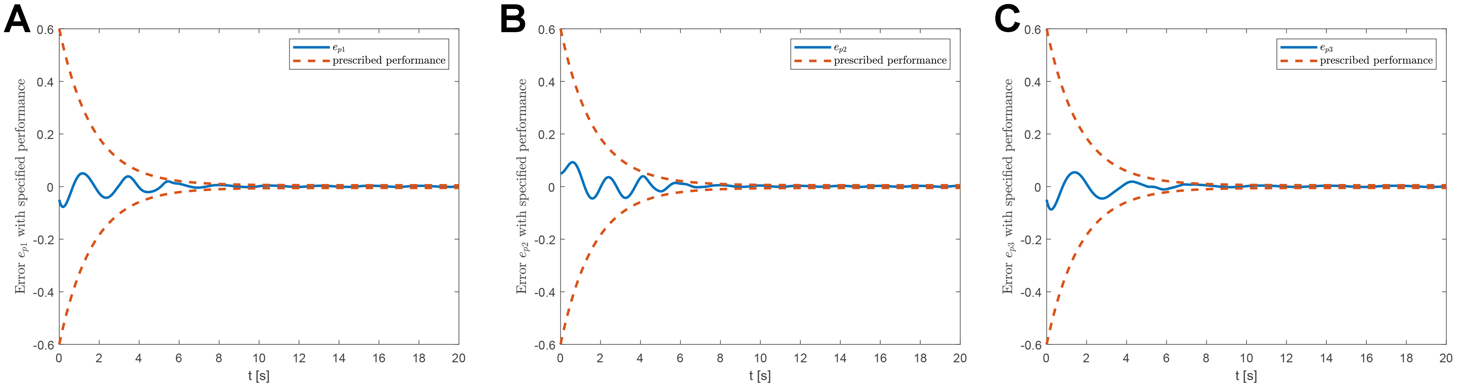
Figure 2. Tracking errors with prescribed performance under the proposed RL-based fault-tolerant attitude controller. (A) Attitude tracking error $$ e_{p1} $$; (B) Attitude tracking error $$ e_{p2} $$ (the dashed lines indicate the prescribed performance boundaries); (C) Attitude tracking error $$ e_{p3} $$. RL: Reinforcement learning.

Reinforcement learning-based attitude control for a quadrotor UAV system with performance constraints

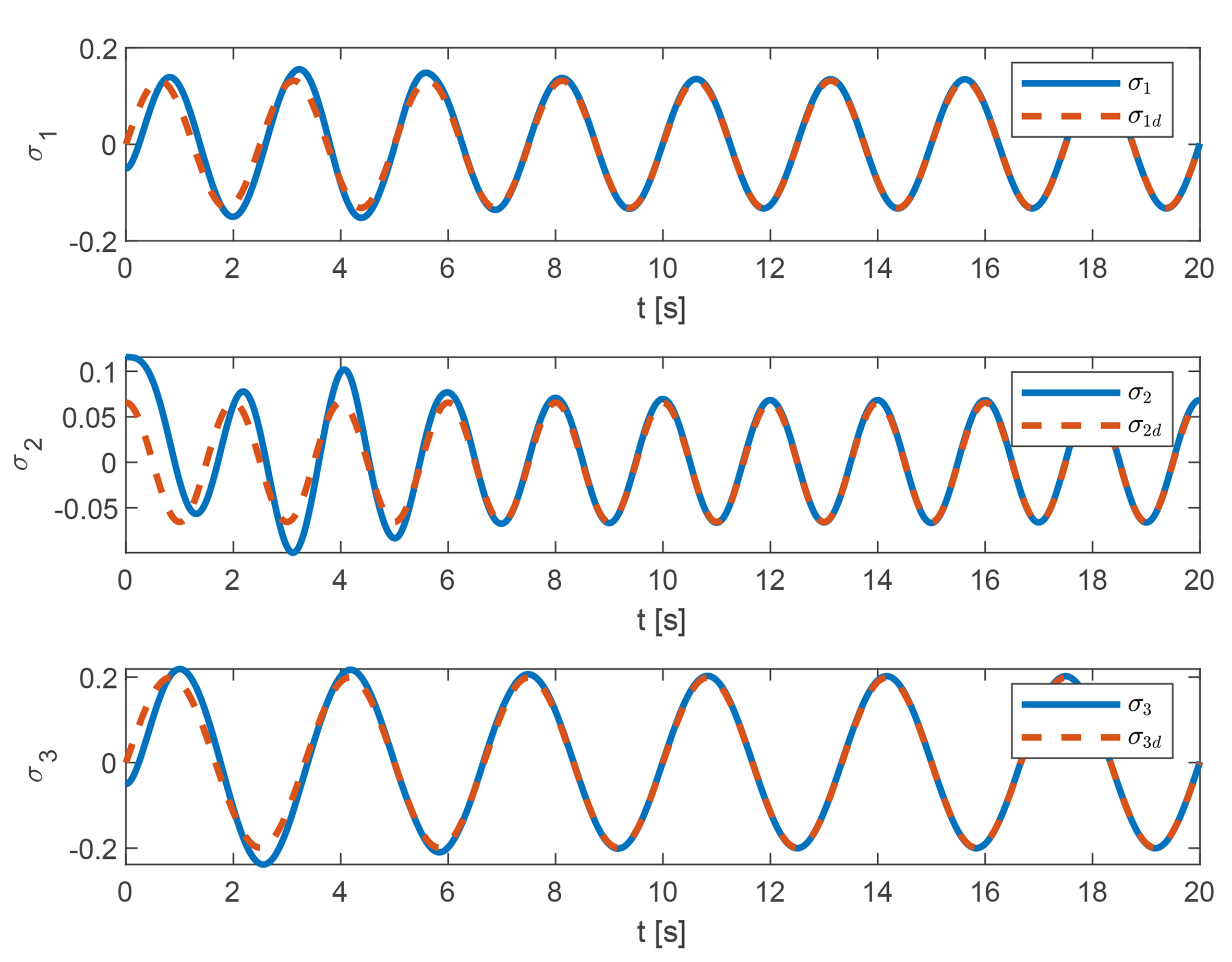
Figure 3. Attitude tracking performance under the proposed RL-based fault-tolerant attitude controller. RL: Reinforcement learning.

Reinforcement learning-based attitude control for a quadrotor UAV system with performance constraints

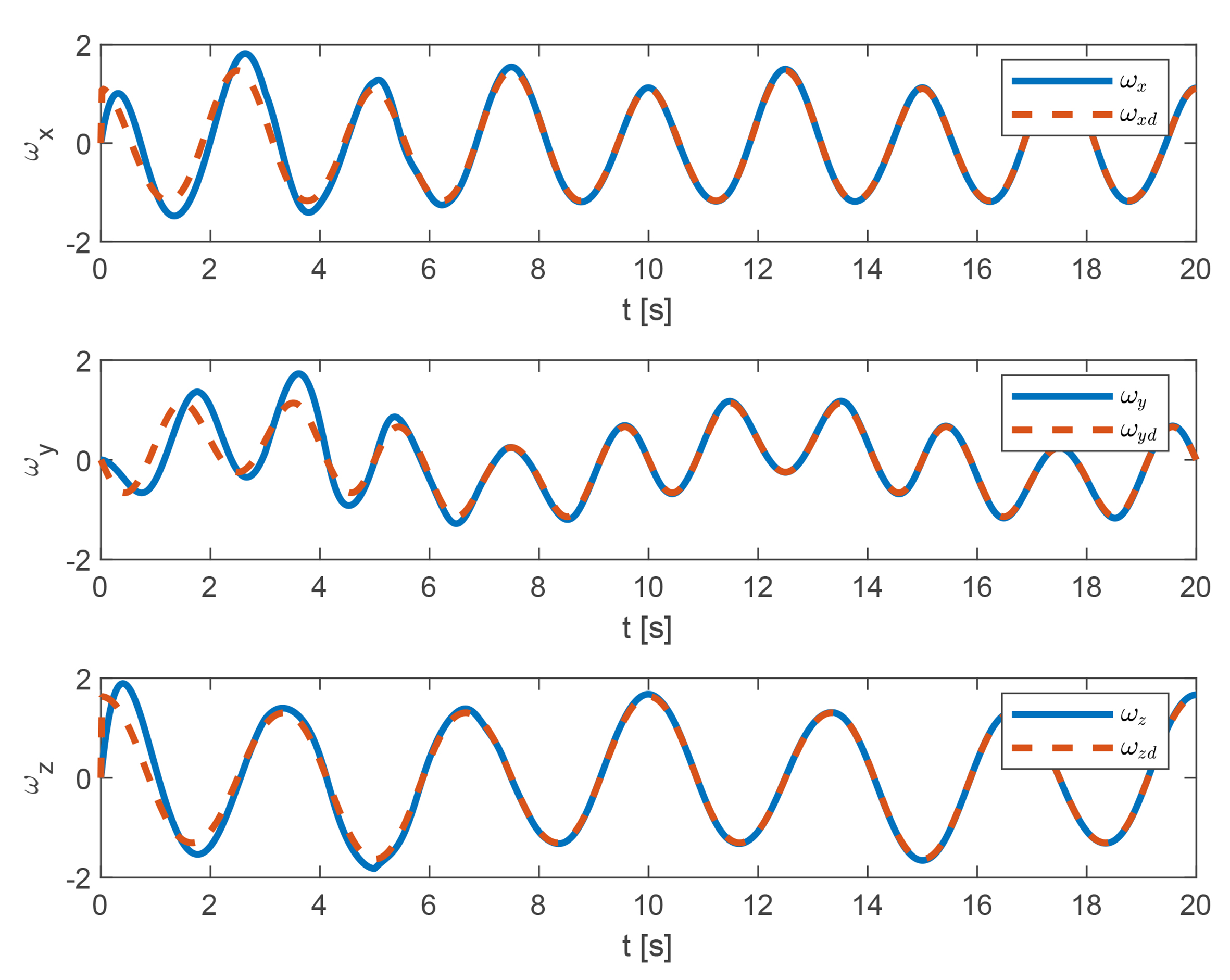
Figure 4. Angular velocity tracking performance of the quadrotor UAV. UAV: Unmanned aerial vehicle.

Reinforcement learning-based attitude control for a quadrotor UAV system with performance constraints

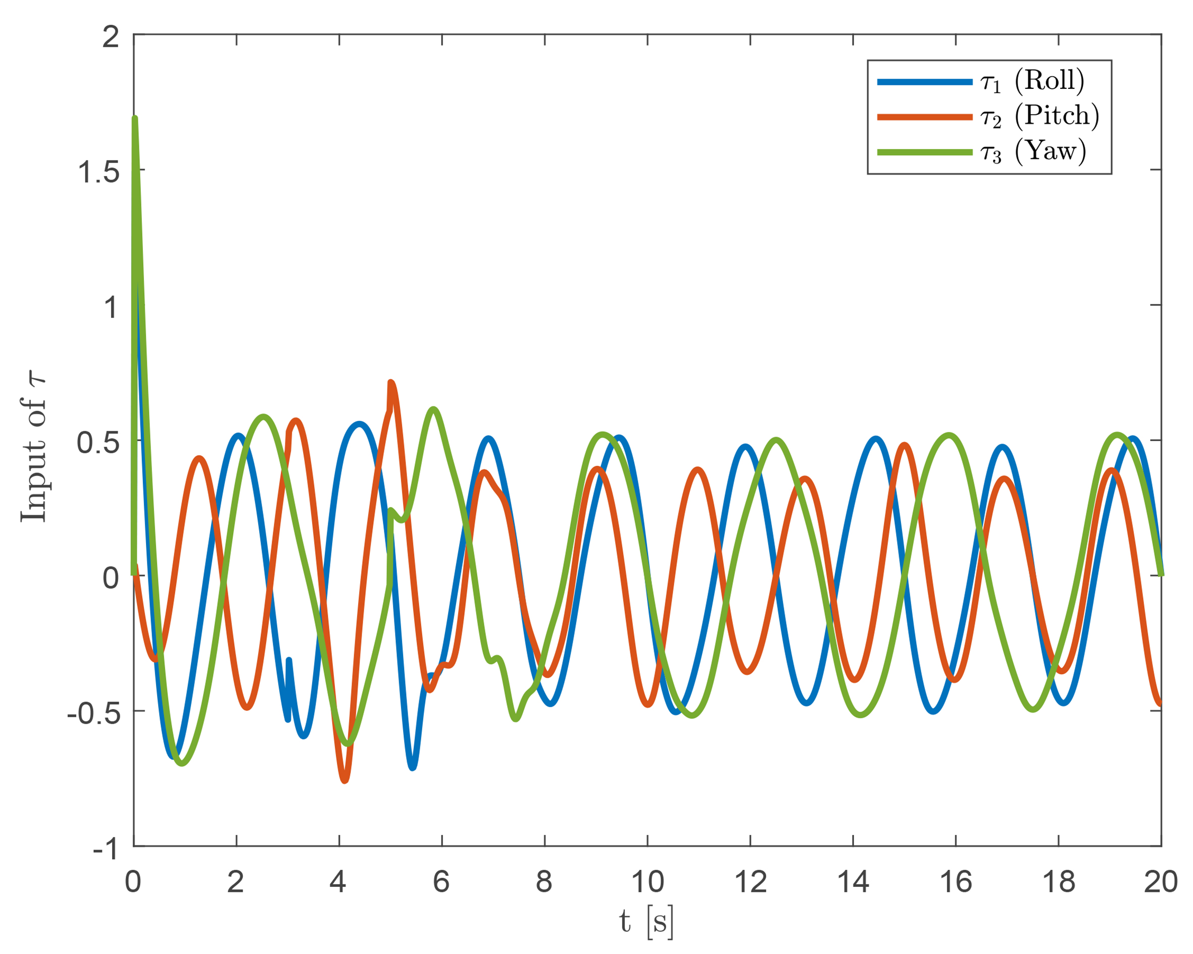
Figure 5. Control torque variation of the quadrotor UAV. UAV: Unmanned aerial vehicle.

Reinforcement learning-based attitude control for a quadrotor UAV system with performance constraints

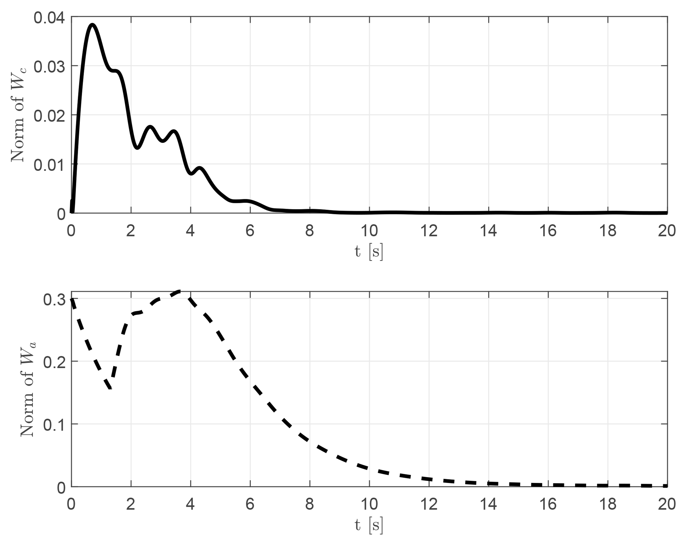
Figure 6. Norms of the critic and actor weight vectors ($$ W_c $$ and $$ W_a $$).

Figure 3 shows the overall tracking performance of the UAV system after attitude angle transformation. The variables $$ \sigma_1 $$ (roll) and $$ \sigma_3 $$ (yaw) achieve satisfactory tracking performance after about 4 s, while $$ \sigma_2 $$ (pitch) attains favorable tracking performance after about 6 s. Figure 4 presents the tracking performance of the quadrotor UAV angular velocity in three coordinate directions. After 6 s, the angular velocity errors converge to a small neighborhood of zero. The input torque of the UAV system is shown in Figure 5, indicating that the control input is reasonable under the considered simulation conditions. Figure 6 shows the norms of the critic and actor weight vectors, reflecting the overall convergence performance of the weights.

To further demonstrate the superiority of the proposed RL-based fault-tolerant attitude control scheme, a conventional proportional-integral-derivative (PID) controller is implemented as a baseline for comparison on a quadrotor UAV system subject to performance constraints and actuator faults. The control torque $$ \tau_{pid} $$ is designed as $$ \tau_{pid} = - K_p e_p(t) - K_i \int_{0}^{t} e_p(\delta) d\delta - K_d \dot{e}_p(t) $$, where $$ e_p(t) $$ denotes the attitude tracking error. The controller gains are selected as $$ K_p = 12I $$, $$ K_d = 5I $$, and $$ K_i = 0.5I $$. The resulting tracking performance is illustrated in Figure 7. As depicted in the figure, the traditional PID controller fails to maintain the tracking errors within the prescribed boundaries after the occurrence of actuator faults, particularly when the performance envelope becomes more restrictive after 5 s. These results highlight that traditional PID control cannot effectively address the attitude tracking problem of the quadrotor UAV system under concurrent actuator failures and stringent performance requirements.

Reinforcement learning-based attitude control for a quadrotor UAV system with performance constraints

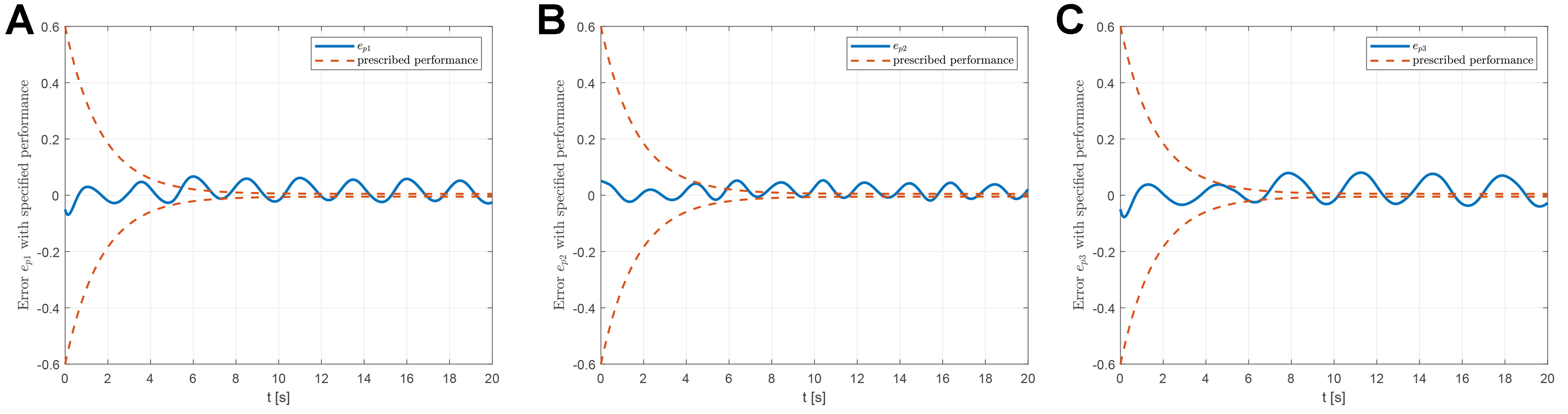
Figure 7. Tracking errors with specified performance under traditional PID control. (A) Attitude tracking error $$ e_{p1} $$; (B) Attitude tracking error $$ e_{p2} $$; (C) Attitude tracking error $$ e_{p3} $$. PID: Proportional-integral-derivative.

For a more rigorous quantitative evaluation, the integral of squared error (ISE) and integral of time-weighted absolute error (ITAE) are calculated and summarized in Table 1. The results show that the proposed method achieves substantially improved tracking performance, with markedly lower ISE values compared to the PID baseline. Notably, the ITAE values obtained by the proposed controller are significantly reduced, indicating that the RL mechanism can suppress transient oscillations caused by actuator faults more rapidly and effectively than conventional control.

Table 1

Quantitative comparison of tracking performance metrics

Metric Control scheme Channel 1 Channel 2 Channel 3
ISE: Integral of squared error; RL: reinforcement learning; PID: proportional-integral-derivative; ITAE: integral of time-weighted absolute error.
ISE Proposed RL-based fault-tolerant attitude control 0.0060 0.0089 0.0072
Traditional PID 0.0219 0.0131 0.0336
ITAE Proposed RL-based fault-tolerant attitude control 0.6799 0.6817 0.6691
Traditional PID 5.5052 4.0884 7.3136

To verify the effectiveness and feasibility of the proposed RL-based fault-tolerant attitude control scheme, comparative simulations are conducted under three scenarios: (1) fault-tolerant control with actuator faults; (2) fault-free control; and (3) control without fault-tolerant under faults. The tracking results for these scenarios are presented in Figures 810. The proposed controller achieves accurate tracking despite the presence of actuator faults, with behavior closely matching the fault-free case. In contrast, the uncompensated faulty system exhibits noticeable tracking errors. These results demonstrate the capability of the fault-tolerant strategy to compensate for actuator faults and maintain reliable tracking performance.

Reinforcement learning-based attitude control for a quadrotor UAV system with performance constraints

Figure 8. Tracking performance of $$ \sigma_1 $$ under different fault conditions.

Reinforcement learning-based attitude control for a quadrotor UAV system with performance constraints

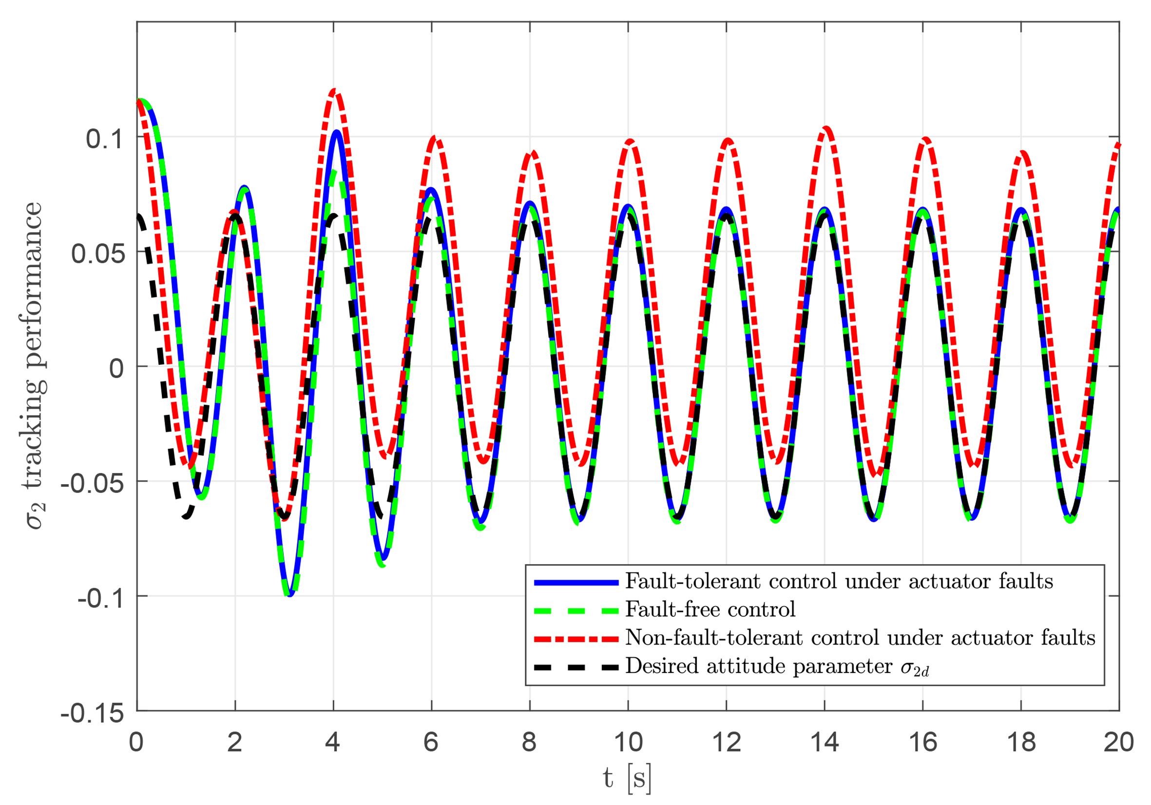
Figure 9. Tracking performance of $$ \sigma_2 $$ under different fault conditions.

Reinforcement learning-based attitude control for a quadrotor UAV system with performance constraints

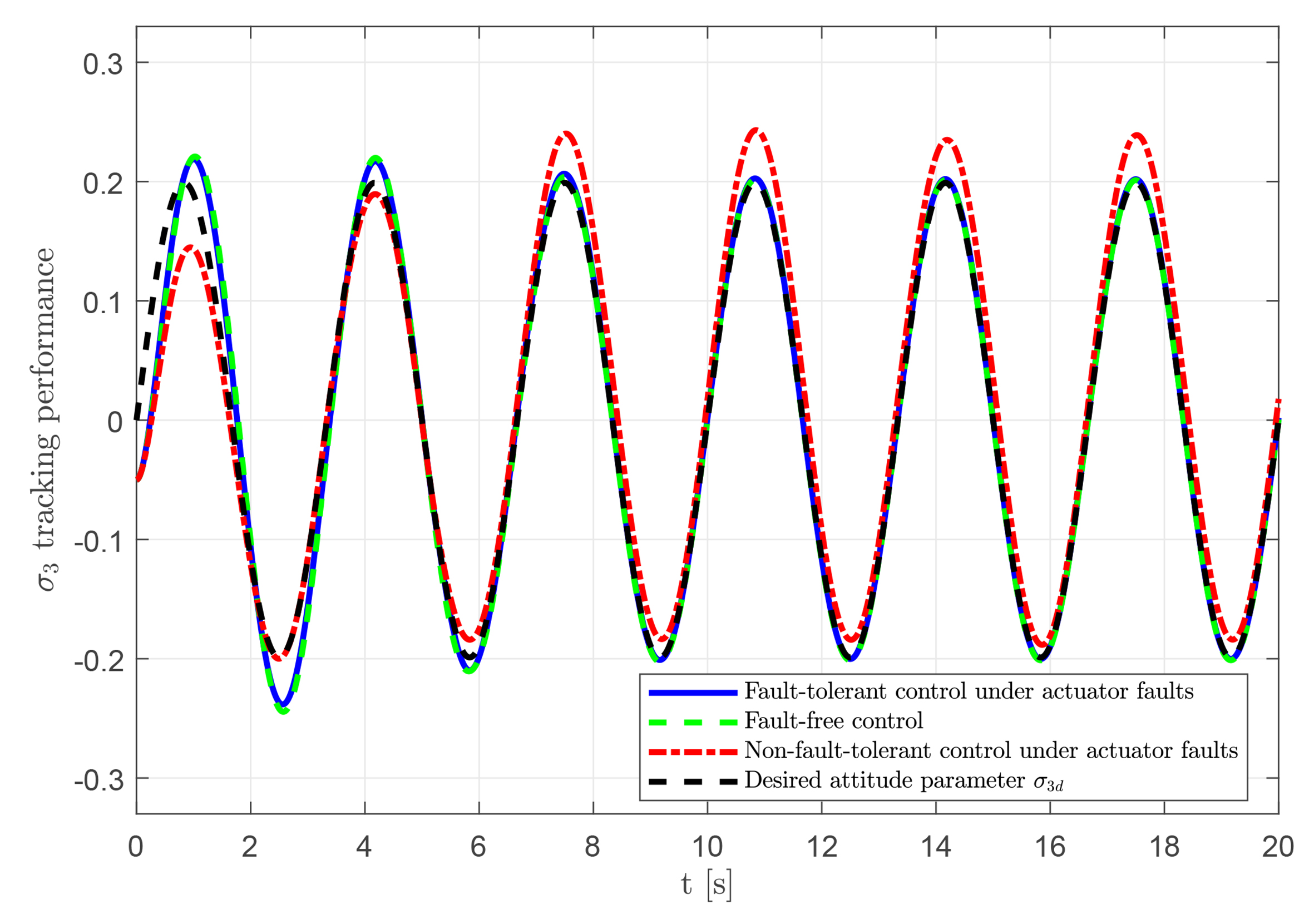
Figure 10. Tracking performance of $$ \sigma_3 $$ under different fault conditions.

In addition, the designed control signal is compared with the actual control input applied, as shown in Figure 11. It can be observed that the control torque remains relatively stable under fault-free conditions. When actuator malfunctions occur at 3 and 5 s, the torque is quickly compensated to maintain system stability. These results indicate that the proposed controller remains effective both in the presence and absence of actuator faults. To investigate the influence of varying design parameters, we further examine the relationship between parameter selection and control performance. Some results are shown in Figures 12 and 13. Specifically, Figure 12A-C illustrate the tracking error comparisons for $$ e_{p1} $$, $$ e_{p2} $$, and $$ e_{p3} $$, respectively, under different parameter configurations. Based on Figure 12, when the critic update parameters are set to $$ \rho_c=0.1 $$ and $$ \xi_c=1 $$, the tracking performance exhibits only marginal differences compared to the original results and remains within a satisfactory range. Furthermore, in contrast to the original results, the performance obtained with $$ \rho_a=30 $$ and $$ \xi_a=0.01 $$ indicates that inappropriate choices of weight update parameters can lead to deteriorated control performance. Therefore, the careful selection of these parameters is crucial for achieving superior control performance.

Reinforcement learning-based attitude control for a quadrotor UAV system with performance constraints

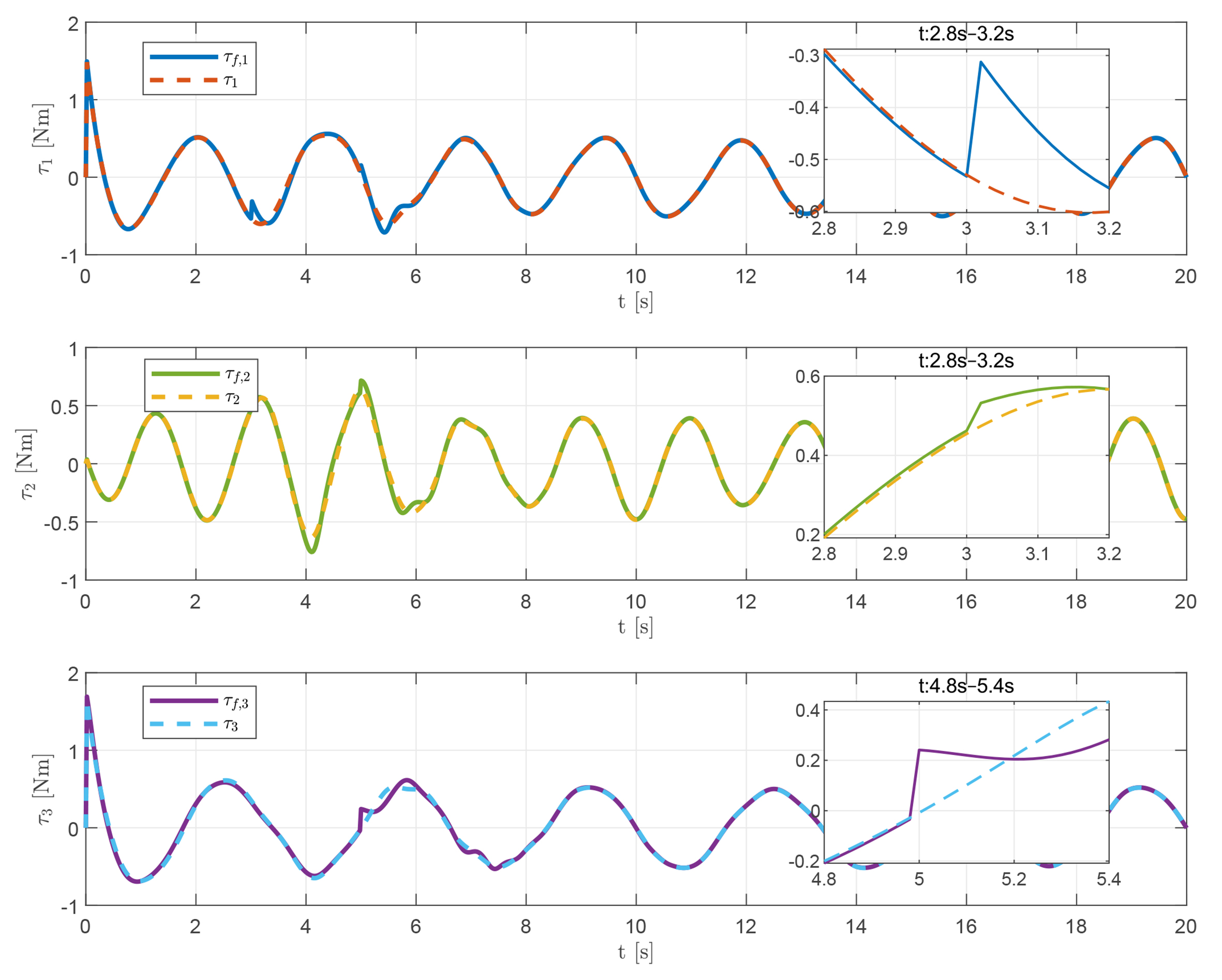
Figure 11. Comparison between the actual control input $$ \tau_f $$ and the designed control signal $$ \tau $$.

Reinforcement learning-based attitude control for a quadrotor UAV system with performance constraints

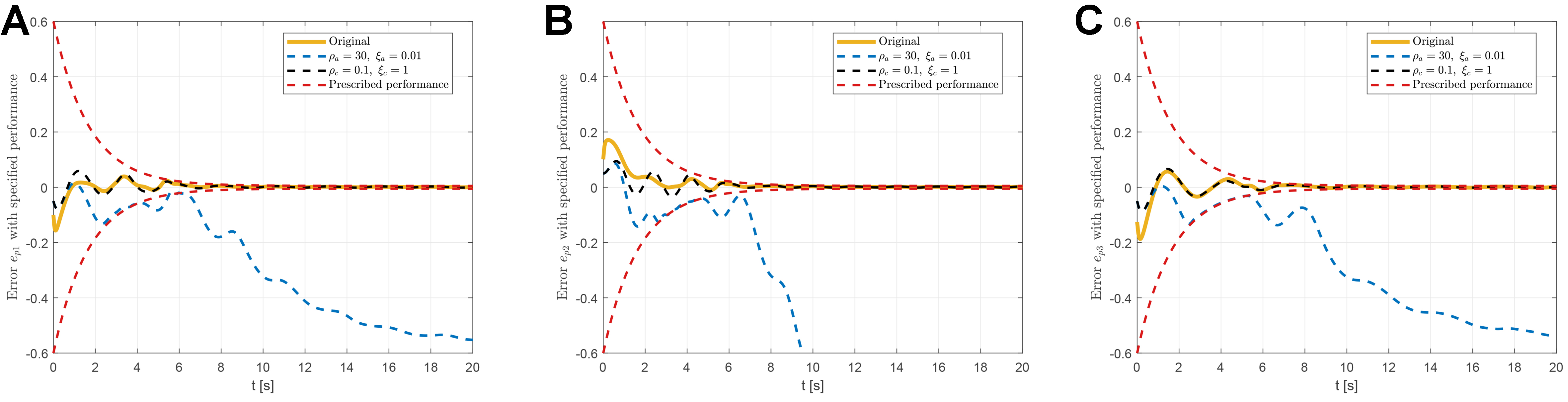
Figure 12. Impact of updating law parameters on attitude tracking performance: (A) tracking error $$ e_{p1} $$ under different parameter settings; (B) tracking error $$ e_{p2} $$ under different parameter settings; (C) tracking error $$ e_{p3} $$ under different parameter settings.

Reinforcement learning-based attitude control for a quadrotor UAV system with performance constraints

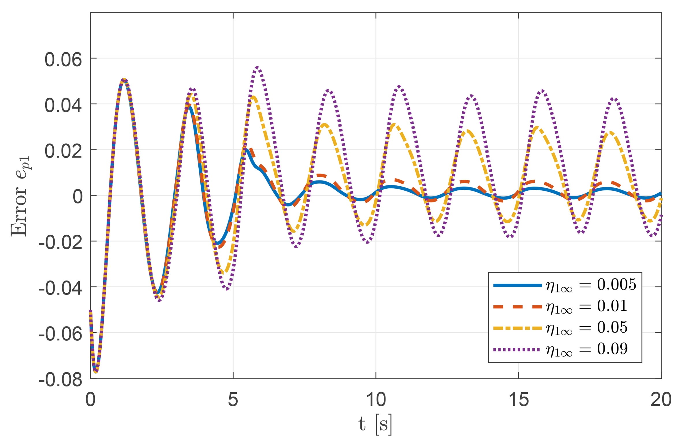
Figure 13. Attitude tracking error $$ e_{p1} $$ under different prescribed performance constraints $$ \eta_{1\infty} $$.

Additionally, as shown in Figure 13, the tracking performance of the UAV system can be guaranteed under appropriately selected prescribed performance parameters. Conversely, when $$ \eta_{1\infty}=0.09 $$, as shown in Figure 13, the tracking errors fail to satisfy the control performance requirements. The above simulation results demonstrate that through the proposed RL-based fuzzy adaptive fault-tolerant attitude control, the UAV system with actuator faults not only exhibits favorable attitude tracking performance, but also satisfies the prescribed performance constraints.

5. CONCLUSIONS

In this paper, a RL-based fuzzy logic fault-tolerant attitude control strategy is proposed for a quadrotor UAV system subject to prescribed performance requirements and actuator faults. To satisfy the performance constraints, a smooth error transformation is introduced to ensure that the tracking errors remain within the desired limits. Within the AC architecture-based RL algorithm, in the critic component, an FLS is used to approximate the value function for performance evaluation and to provide a reinforcement signal. In the actor component, an FLS is employed to generate the control input based on the reinforcement signal. With the proposed fuzzy adaptive fault-tolerant attitude control scheme, the stability of the closed-loop UAV system is guaranteed using Lyapunov stability theory, even in the presence of system uncertainties, performance constraints, and actuator faults. Finally, simulations of the quadrotor UAV system are conducted, and the results demonstrate that the proposed RL-based fuzzy adaptive fault-tolerant attitude control strategy is effective and feasible.

DECLARATIONS

Authors' contributions

Conceived the research concept, designed the methodology, established the simulation platform, drafted the original manuscript, prepared the visualizations, and obtained funding support: Ouyang, Y.

Participated in data analysis, performed the main simulations, conducted simulation validation, contributed to drafting the original manuscript, and revised the manuscript: Ma, C.

Conducted data curation, assisted in result analysis, performed data visualization, and polished the manuscript: Wang, Y.

Provided technical support, assisted in establishing the simulation platform, and revised the manuscript: Su, Y.

Supervised the entire project, managed project administration, thoroughly reviewed and edited the manuscript, and validated all results: He, X.

Availability of data and materials

The data supporting the findings of this study are available from the corresponding author upon reasonable request.

AI and AI-assisted tools statement

Not applicable.

Financial support and sponsorship

This work was supported by the National Natural Science Foundation of China (Grant Nos. 62303008, 62303012, 62495083, and 62236002).

Conflicts of interest

All authors declared that there are no conflicts of interest.

Ethical approval and consent to participate

Not applicable.

Consent for publication

Not applicable.

Copyright

© The Author(s) 2026.

REFERENCES

1. Huang, H.; He, W.; Chen, Z.; Niu, T.; Fu, Q. Development and experimental characterization of a robotic butterfly with a mass shifter mechanism. Biomimetic. Intell. Robot. 2022, 2, 100076.

2. He, W.; Mu, X.; Zhang, L.; Zou, Y. Modeling and trajectory tracking control for flapping-wing micro aerial vehicles. IEEE/CAA. J. Autom. Sin. 2021, 8, 148-56.

3. Wu, C.; Xiao, Y.; Zhao, J.; Cui, F.; Wu, X.; Liu, W. JingWei: a waterfowl-inspired flapping-wing robot with multimodal aerial-aquatic mobility. IEEE. Robot. Autom. Lett. 2025, 10, 11046-53.

4. Chen, Y.; Pérez-Arancibia, N. O. Adaptive control of a VTOL uncrewed aerial vehicle for high-performance aerobatic flight. Automatica 2024, 159, 109922.

5. Zheng, Z.; Li, J.; Guan, Z.; Zuo, Z. Constrained moving path following control for UAV with robust control barrier function. IEEE/CAA. J. Autom. Sin. 2023, 10, 1557-70.

6. Xu, B.; Suleman, A.; Shi, Y. A multi-rate hierarchical fault-tolerant adaptive model predictive control framework: theory and design for quadrotors. Automatica 2023, 153, 111015.

7. Dong, F.; Yuan, B.; Zhao, X.; Ding, Z.; Chen, S. Adaptive robust constraint-following control for morphing quadrotor UAV with uncertainty: a segmented modeling approach. J. Franklin. Inst. 2024, 361, 106678.

8. Zhao, Z.; Zhang, J.; Liu, Z.; He, W.; Hong, K. S. Adaptive quantized fault-tolerant control of a 2-DOF helicopter system with actuator fault and unknown dead zone. Automatica 2023, 148, 110792.

9. Zhao, W.; Liu, H.; Lewis, F. L. Data-driven fault-tolerant control for attitude synchronization of nonlinear quadrotors. IEEE. Trans. Autom. Control. 2021, 66, 5584-91.

10. Liu, Y.; Dong, X.; Shi, P.; Ren, Z.; Liu, J. Distributed fault-tolerant formation tracking control for multiagent systems with multiple leaders and constrained actuators. IEEE. Trans. Cybern. 2023, 53, 3738-47.

11. Ma, Y.; Jiang, B.; Wang, J.; Gong, J. Adaptive fault-tolerant formation control for heterogeneous UAVs-UGVs systems with multiple actuator faults. IEEE. Trans. Aerosp. Electron. Syst. 2023, 59, 6705-16.

12. Hu, Y.; Yan, H.; Wang, M.; Hu, X.; Li, Z. Fuzzy observer-based input/output event-triggered control for Euler–lagrange systems with guaranteed performance and input saturation. IEEE. Trans. Fuzzy. Syst. 2024, 32, 2077-88.

13. Ren, Y.; Sun, Y.; Liu, Z.; Lam, H. K. Parameter-optimization-based adaptive fault-tolerant control for a quadrotor UAV using fuzzy disturbance observers. IEEE. Trans. Fuzzy. Syst. 2025, 33, 593-605.

14. Kong, L.; He, W.; Yang, C.; Li, Z.; Sun, C. Adaptive fuzzy control for coordinated multiple robots with constraint using impedance learning. IEEE. Trans. Cybern. 2019, 49, 3052-63.

15. Zhang, F.; Dai, P.; Na, J.; Gao, G.; Shi, Y.; Liu, F. Adaptive fuzzy tracking control for a class of uncertain nonlinear systems with improved prescribed performance. IEEE. Trans. Fuzzy. Syst. 2025, 33, 1133-45.

16. Yu, D.; Ma, S.; Liu, Y. J.; Wang, Z.; Chen, C. L. P. Finite-time adaptive fuzzy backstepping control for quadrotor UAV with stochastic disturbance. IEEE. Trans. Autom. Sci. Eng. 2024, 21, 1335-45.

17. Su, M.; Pu, R.; Wang, Y.; Yu, M. A collaborative siege method of multiple unmanned vehicles based on reinforcement learning. Intell. Robot. 2024, 4, 39-60.

18. Dong, L.; He, Z.; Song, C.; Sun, C. A review of mobile robot motion planning methods: from classical motion planning workflows to reinforcement learning-based architectures. J. Syst. Eng. Electron. 2023, 34, 439-59.

19. Zhang, H.; He, L.; Wang, D. Deep reinforcement learning for real-world quadrupedal locomotion: a comprehensive review. Intell. Robot. 2022, 2, 275-97.

20. Wen, G.; Yu, D.; Zhao, Y. Optimized fuzzy attitude control of quadrotor unmanned aerial vehicle using adaptive reinforcement learning strategy. IEEE. Trans. Aerosp. Electron. Syst. 2024, 60, 6075-83.

21. Wen, G.; Niu, B. Optimized distributed formation control using identifier–critic–actor reinforcement learning for a class of stochastic nonlinear multi-agent systems. ISA. Trans. 2024, 155, 1-10.

22. Han, M.; Zhang, L.; Wang, J.; Pan, W. Actor-critic reinforcement learning for control with stability guarantee. IEEE. Robot. Autom. Lett. 2020, 5, 6217-24.

23. Ouyang, Y.; Xue, L.; Dong, L.; Sun, C. Neural network-based finite-time distributed formation-containment control of two-Layer quadrotor UAVs. IEEE. Trans. Syst. Man. Cybern. Syst. 2022, 52, 4836-48.

24. Ouyang, Y.; Sun, C.; Dong, L. Actor–critic learning based coordinated control for a dual-arm robot with prescribed performance and unknown backlash-like hysteresis. ISA. Trans. 2022, 126, 1-13.

25. Zhou, Z. G.; Zhou, D.; Chen, X.; Shi, X. N. Adaptive actor-critic learning-based robust appointed-time attitude tracking control for uncertain rigid spacecrafts with performance and input constraints. Adv. Space. Res. 2023, 71, 3574-87.

26. Han, H.; Cheng, J.; Xi, Z.; Lv, M. Symmetric actor–critic deep reinforcement learning for cascade quadrotor flight control. Neurocomputing 2023, 559, 126789.

27. Yang, S.; Pan, Y.; Cao, L.; Chen, L. Predefined-time fault-tolerant consensus tracking control for Multi-UAV systems with prescribed performance and attitude constraints. IEEE. Trans. Aerosp. Electron. Syst. 2024, 60, 4058-72.

28. Yu, Z.; Li, J.; Xu, Y.; Zhang, Y.; Jiang, B.; Su, C. Y. Reinforcement learning-based fractional-order adaptive fault-tolerant formation control of networked fixed-wing UAVs with prescribed performance. IEEE. Trans. Neural. Netw. Learn. Syst. 2024, 35, 3365-79.

29. Aforozi, T. A.; Rovithakis, G. A. Prescribed performance tracking for uncertain MIMO pure-feedback systems with unknown and partially nonconstant control directions. IEEE. Trans. Autom. Control. 2024, 69, 7285-92.

30. Wang, X.; Kong, L.; Meng, T.; Xia, J.; He, W. Event-triggered tracking control for a flapping-wing aerial vehicle with prescribed performance. IEEE. Trans. Aerosp. Electron. Syst. 2025, 61, 17476-87.

31. Li, Z.; Wang, X.; Guo, H.; Xi, L.; Liu, G.; Li, Y. Distributed output feedback prescribed performance control for high-order nonlinear multi-agent systems. IEEE. Trans. Autom. Sci. Eng. 2025, 22, 12730-40.

32. Li, D.; Ma, G.; Li, C.; He, W.; Mei, J.; Ge, S. S. Distributed attitude coordinated control of multiple spacecraft with attitude constraints. IEEE. Trans. Aerosp. Electron. Syst. 2018, 54, 2233-45.

33. Ouyang, Y.; Dong, L.; Wei, Y.; Sun, C. Neural network based tracking control for an elastic joint robot with input constraint via actor-critic design. Neurocomputing 2020, 409, 286-95.

34. Wang, X.; Wang, Q.; Sun, C. Prescribed performance fault-tolerant control for uncertain nonlinear MIMO system using actor–critic learning structure. IEEE. Trans. Neural. Netw. Learn. Syst. 2022, 33, 4479-90.

35. Guo, X.; Yan, W.; Cui, R. Integral reinforcement learning-based adaptive NN control for continuous-time nonlinear MIMO systems with unknown control directions. IEEE. Trans. Syst. Man. Cybern. Syst. 2020, 50, 4068-77.

Cite This Article

Research Article
Open Access
Reinforcement learning-based attitude control for a quadrotor UAV system with performance constraints

How to Cite

Download Citation

If you have the appropriate software installed, you can download article citation data to the citation manager of your choice. Simply select your manager software from the list below and click on download.

Export Citation File:

Type of Import

Tips on Downloading Citation

This feature enables you to download the bibliographic information (also called citation data, header data, or metadata) for the articles on our site.

Citation Manager File Format

Use the radio buttons to choose how to format the bibliographic data you're harvesting. Several citation manager formats are available, including EndNote and BibTex.

Type of Import

If you have citation management software installed on your computer your Web browser should be able to import metadata directly into your reference database.

Direct Import: When the Direct Import option is selected (the default state), a dialogue box will give you the option to Save or Open the downloaded citation data. Choosing Open will either launch your citation manager or give you a choice of applications with which to use the metadata. The Save option saves the file locally for later use.

Indirect Import: When the Indirect Import option is selected, the metadata is displayed and may be copied and pasted as needed.

About This Article

Special Topic

Disclaimer/Publisher’s Note: All statements, opinions, and data contained in this publication are solely those of the individual author(s) and contributor(s) and do not necessarily reflect those of OAE and/or the editor(s). OAE and/or the editor(s) disclaim any responsibility for harm to persons or property resulting from the use of any ideas, methods, instructions, or products mentioned in the content.
© The Author(s) 2026. Open Access This article is licensed under a Creative Commons Attribution 4.0 International License (https://creativecommons.org/licenses/by/4.0/), which permits unrestricted use, sharing, adaptation, distribution and reproduction in any medium or format, for any purpose, even commercially, as long as you give appropriate credit to the original author(s) and the source, provide a link to the Creative Commons license, and indicate if changes were made.

Data & Comments

Data

Views
60
Downloads
5
Citations
0
Comments
0
2

Comments

Comments must be written in English. Spam, offensive content, impersonation, and private information will not be permitted. If any comment is reported and identified as inappropriate content by OAE staff, the comment will be removed without notice. If you have any queries or need any help, please contact us at [email protected].

0
Download PDF
Share This Article
Scan the QR code for reading!
See Updates
Contents
Figures
Related
Intelligence & Robotics
ISSN 2770-3541 (Online)

Portico

All published articles are preserved here permanently:

https://www.portico.org/publishers/oae/

Portico

All published articles are preserved here permanently:

https://www.portico.org/publishers/oae/